Fluid-flow theory

The FluidFlow code is responsible for providing Ross with simulations of thin thickness fluid in hydrodynamic bearings. It returns relevant information for the stability analysis of rotating machines, such as pressure field, fluid forces and dynamic coefficients. In this section, the main theoretical foundations of the modeling described in the code are synthesized and some examples are provided.

import ross
from ross.fluid_flow.fluid_flow import fluid_flow_example2

my_fluid_flow = fluid_flow_example2()

PROBLEM DESCRIPTION

Fluid flow occurs in the annular space between the shaft and the bearing, both of \( L \) length. These structures are called rotor and stator, respectively. The stator is fixed with radius \(R_{o}\) and the rotor, with radius \(R_{i} \), is a rigid body with rotation speed \(\omega\), as shown in the figure below.

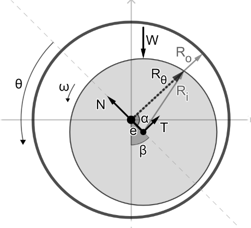
Due to the rotation of the rotor, a pressure field is set in the lubricating oil film, developing fluid forces that act on the rotor surface. For a constant speed of rotation, these forces displace the rotor to a location inside the stator called the equilibrium position. In this position, the stator and rotor are eccentric, with a distance between centers \(e\) and an attitude angle \(\beta\), formed between the axis connecting both centers and the vertical axis.

Based on the eccentricity and attitude angle, the cosine law can be used to describe the position of the rotor surface \(R_{\theta}\) with respect to the center of the stator:

\[ R_{\theta} = \sqrt{R_i ^2 - e^2 \sin^2{\alpha}} + e \cos{\alpha},\]

where $\alpha =\begin{cases} \dfrac{3\pi}{2} - \theta + \beta \text{,} &\mbox{se } \dfrac{\pi}{2} + \beta \leq \theta < \dfrac{3\pi}{2} + \beta \ \

• \left(\dfrac{3\pi}{2} - \theta + \beta\right) \text{,} & \mbox{se } \dfrac{3\pi}{2} + \beta \leq \theta < \dfrac{5\pi}{2} + \beta \end{cases}$.

from ross.fluid_flow.fluid_flow_graphics import plot_eccentricity

fig = plot_eccentricity(my_fluid_flow, z=int(my_fluid_flow.nz / 2), scale_factor=0.5)
fig.show()

THEORETICAL MODELING

We start from the Navier Stokes and continuity equations:

\[\rho \left(\dfrac{\partial \mathbf{v}}{\partial t} + \mathbf{v} \cdot \nabla \mathbf{v} \right) = \nabla \cdot \sigma\]

\[\dfrac{\partial \rho}{\partial t} + \nabla \cdot \left( \rho \mathbf{v} \right) = 0\]

where \(\rho\) is the specific mass of the fluid, \(\mathbf{v}\) is the velocity field, and \(\sigma=-p \mathbf{I} + \tau\) is the Cauchy’s tensor, in which \(p\) represents the pressure field, \(\tau\) is the stress tensor and \(\mathbf{I}\) the identity tensor. In order to consider the effects of curvature, the velocity field is represented in cylindrical coordinates with \(u\), \(v\) and \(w\) being the axial, radial and tangential speeds, respectively.

In this code, the following hypotheses are considered:

• Newtonian fluid: \({\mathbf{\tau}} = {\mathbf{\mu}}(\nabla \mathbf{v})\)

• Incompressible fluid: constant \(\rho\)

• Permanent regime: \(\dfrac{\partial(*)}{\partial t}=0\)

Thus, the equations can be rewritten as

\[\rho \left(\mathbf{v} \cdot \nabla \mathbf{v}\right) = - \nabla p + \mu \nabla^2 \mathbf{v}\]

\[\nabla \cdot \mathbf{v}=0,\]

or in terms of each direction:

• Direction \(z\) (similar to directions \(r\) and \(\theta\)):

\[{\rho \left( u \dfrac{\partial{u}}{\partial{z}} + v \dfrac{\partial{u}}{\partial{r}} + \dfrac{w}{r} \dfrac{\partial{u}}{\partial{\theta}} \right)} = {-\dfrac{\partial{p}}{\partial{z}} + \mu \left( \dfrac{1}{r} \dfrac{\partial{}}{\partial{r}}\left[r\dfrac{\partial{u}}{\partial{r}} \right] + \dfrac{1}{r^2}\dfrac{\partial^2{u}}{\partial{\theta ^2}} + \dfrac{\partial^2{u}}{\partial{z^2}} \right)}\]

• Continuity:

\[\dfrac{1}{r} \dfrac{\partial{\left(rv\right)}}{\partial{r}}+\dfrac{1}{r}\dfrac{\partial{w}}{\partial{\theta}}+\dfrac{\partial{u}}{\partial{z}} = 0\]

Dimensionaless Analysis

Considering U and L as a typical speed and sizes with the relation

\[(R_{o}-R_{i}) = F \ll L,\]

the equation that represents movement in the \(z\) direction, in its dimensionless form, is:

\[{\rho \left( U\hat{u} \dfrac{\partial{U\hat{u}}}{\partial{L\hat{z}}} + U\hat{v} \dfrac{\partial{U\hat{u}}}{\partial{F\hat{r}}} + \dfrac{U\hat{w}}{L\hat{r}} \dfrac{\partial{U\hat{u}}}{\partial{\theta}} \right)} = {-\dfrac{\partial{P\hat{p}}}{\partial{L\hat{z}}} + \mu \left( \dfrac{1}{L\hat{r}} \dfrac{\partial{}}{\partial{F\hat{r}}}\left[L\hat{r}\dfrac{\partial{U\hat{u}}}{\partial{F\hat{r}}} \right] + \dfrac{1}{L^2\hat{r}^2}\dfrac{\partial^2{U\hat{u}}}{\partial{\theta ^2}} + \dfrac{\partial^2{U\hat{u}}}{\partial{L^2\hat{z}^2}} \right)}\]

where the dimensionless quantities aare denoted with a circumflex accent.

The previous equation is rearranged to explicit the Reynolds number \(\left(\mathbf{Re}=\dfrac{\rho U L}{\mu}\right)\) by using the relation \(P = \dfrac{\mu UL}{F^2}\):

\[{ \mathbf{Re} \left( \left(\dfrac{F^2}{L^2}\right)\hat{u} \dfrac{\partial{\hat{u}}}{\partial{\hat{z}}} + \left(\dfrac{F}{L} \right) \hat{v} \dfrac{\partial{\hat{u}}}{\partial{\hat{r}}} + \left(\dfrac{F^2}{L^2}\right) \dfrac{\hat{w}}{\hat{r}} \dfrac{\partial{\hat{u}}}{\partial{\theta}} \right)} = {-\dfrac{\partial{\hat{p}}}{\partial{\hat{z}}} + \left( \dfrac{1}{\hat{r}} \dfrac{\partial{}}{\partial{\hat{r}}}\left[\hat{r}\dfrac{\partial{\hat{u}}}{\partial{\hat{r}}} \right] + \left(\dfrac{F^2}{L^2}\right) \dfrac{1}{\hat{r}^2}\dfrac{\partial^2{\hat{u}}}{\partial{\theta ^2}} + \left(\dfrac{F^2}{L^2}\right)\dfrac{\partial^2{\hat{u}}}{\partial{\hat{z}^2}} \right)}\]

After some simplifications, based on lubrication theory, the equations along each direction are:

• \(z\) direction:

\[-\dfrac{\partial{\hat{p}}}{\partial{\hat{z}}} + \dfrac{1}{\hat{r}} \dfrac{\partial{}}{\partial{\hat{r}}}\left(\hat{r}\dfrac{\partial{\hat{u}}}{\partial{\hat{r}}} \right) =0\]

• \(r\) direction:

\[-\dfrac{\partial{\hat{p}}}{\partial{\hat{r}}}=0\]

• \(\theta\) direction:

\[\dfrac{\partial{}}{\partial{\hat{r}}} \left(\dfrac{1}{\hat{r}}\dfrac{\partial{(\hat{r}\hat{w})}}{\partial{\hat{r}}}\right) - \dfrac{1}{\hat{r}}\dfrac{\partial{\hat{p}}}{\partial{\theta}} =0\]

Returning to the dimensional form and noting that the pressure does not change along the radial direction, the simplified Reynold’s equations are:

\[-\dfrac{\partial{p}}{\partial{z}} + \mu \left[\dfrac{1}{r} \dfrac{\partial{}}{\partial{r}}\left(r\dfrac{\partial{u}}{\partial{r}} \right)\right] =0\]

\[-\dfrac{1}{r} \dfrac{\partial{p}}{\partial{\theta}} + \mu \left[\dfrac{\partial{}}{\partial{r}}\left(\dfrac{1}{r}\dfrac{\partial{(rw)}}{\partial{r}}\right)\right] =0\]

Speeds

It is now possible to integrate the above equations to find the velocities in the \(z\) (axial velocity \(u\)) and \(\theta\) (tangential velocity w) directions. This yields:

\[u = \dfrac{1}{\mu}\left[\dfrac{\partial{p}}{\partial{z}}\dfrac{r^2}{4} + c_1 \ln{r} + c_2\right]\]

\[w = \dfrac{1}{\mu} \left\{\dfrac{1}{2}\left[\dfrac{\partial{p}}{\partial{\theta}} r \left(\ln{r} -\dfrac{1}{2}\right) + c_3 r\right] + \dfrac{c_4}{r}\right\}\]

where \(c_1\), \(c_2\), \(c_3\) and \(c_4\) are constant in the integration in the variable \(r\).

By applying the boundary conditions

• \(u(R_{o})=u(R_{\theta})=0,\)

• \(w(R_{o})=0\) and \(w(R_{\theta}) = \omega R_{i},\)

the speeds are

\[u = \dfrac{1}{4\mu} \dfrac{\partial{p}}{\partial{z}} R_{\theta}^2 \left[ \left( \dfrac{r}{R_{\theta}} \right)^2 - \dfrac{\left(R_{o}^2 - R_{\theta}^2\right)}{R_{\theta}^2 \ln{\left(\dfrac{R_{o}}{R_{\theta}}\right)}} \left( \ln{\dfrac{r}{R_{\theta}}} \right) - 1 \right]\]

\[w = \dfrac{1}{2 \mu} \dfrac{\partial p}{\partial \theta} \left[ r \left( \ln r - \dfrac{1}{2} \right) + k r - \dfrac{R_{o}^2}{r} \left( \ln R_{o} + k - \dfrac{1}{2} \right) \right] + \dfrac{\omega R_{i} R_{\theta}}{\left(R_{\theta}^2 - R_{o}^2\right)} \left( r - \dfrac{R_{o}^2}{r} \right)\]

where \(k = \frac{1}{R^2_{\theta}-R^2_{o}} \left[ R^2_{o} \left( \ln R_{o} - \frac{1}{2} \right) -R^2_{\theta} \left( \ln R_{\theta} - \frac{1}{2} \right) \right]\)

Pressure

Once the speeds are calculated, the continuity equation is integrated into the annular region of interest, from \(R_{\theta}\) to \(R_o\):

\[ \int^{R_{o}}_{R_{\theta}} \left( \frac{\partial{(rv)}}{\partial{r}} + \frac{\partial{w}}{\partial{\theta}} + \frac{\partial{(ru)}}{\partial{z}} \right) \,dr = 0\]

The integral is splitted into three integrals and the fundamental theorem of calculus and Leibnitz rule are applied. This yields:

1. \(\int^{R_{o}}_{R_{\theta}} \left( \frac{\partial{(rv)}}{\partial{r}} \right) \,dr = R_{o} v(R_{o}) - R_{\theta} v(R_{\theta})\)

2. \(\int^{R_{o}}_{R_{\theta}} \left( \frac{\partial{w}}{\partial{\theta}} \right) \, dr = \dfrac{\partial}{\partial \theta} \int^{R_{o}}_{R_{\theta}} w \,dr - \left[ w(R_{o}) \dfrac{\partial R_{o}}{\partial \theta} - w(R_{\theta}) \dfrac{\partial R_{\theta}}{\partial \theta} \right]\)

3. \(\int^{R_{o}}_{R_{\theta}} \left( \frac{\partial{(ru)}}{\partial{z}} \right) \, dr = \dfrac{\partial}{\partial z} \int^{R_{o}}_{R_{\theta}} (ru) \,dr - \left[ u(R_{o}) \dfrac{\partial R_{o}}{\partial z} - u(R_{\theta}) \dfrac{\partial R_i}{\partial z} \right]\)

Here, some considerations are taken into account:

• The radial velocity is zero at \(v(R_{o})=0\). However, \(v(R_{\theta})\neq 0\) because the origin of the frame is not in the center of the rotor.

• As seen earlier, \(w(R_o) = 0\) and \(w(R_{\theta}) = \omega R_{i}\). Due to the eccentricity, \(\dfrac{\partial R_{\theta}}{\partial \theta} \neq 0\).

• By the boundary condition it is known that \(u(R_o)=u(R_{\theta})=0\).

Moreover, the speeds \(v(R_{\theta})\) and \(w(R_{\theta})\) must be calculated with kinematic relations. First, consider any \( A \) point pertaining to the rotor surface. Due to rotation, point \(A\) has a velocity

\[v_{rot} = v_{rad}\,e_{r} + v_{tan}\,e_{\theta},\]

where \(e_{r}\) and \(e_{\theta}\) are unit vectors of the cylindrical coordinate system. This is shown in the figure below.

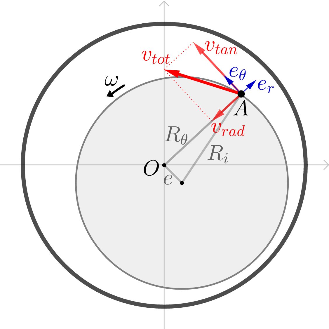
Now, consider the position vector \(a=R_{\theta} e_r\), from the stator center to any point in the rotor surface. Its time derivative, relative to an inertial frame, is the total speed \(v_{tot}\):

\[v_{rot}=\omega \dfrac{\partial R_{\theta}}{\partial \theta}\,e_r + \omega R_{\theta}\,e_{\theta}\]

where \(v(R_{\theta}) = \omega \dfrac{\partial R_{\theta}}{\partial \theta}\) and \(w(R_{\theta}) = \omega R_{\theta}\).

Substituting the values of \(v(R_{\theta})\) and \(w(R_{\theta})\) in the continuity equation, we obtain:

\[\dfrac{\partial}{\partial \theta} \int^{R_{o}}_{R_{\theta}} w \,dr + \dfrac{\partial}{\partial z} \int^{R_{o}}_{R_{\theta}} ru \,dr = 0\]

Performing this integral and replacing the \(u\) and \(w\) speeds yields:

\[\dfrac{\partial}{\partial \theta} \left( \mathbf{C_1} \dfrac{\partial p}{\partial \theta} \right) + \dfrac{\partial}{\partial z} \left( \mathbf{C_2} \dfrac{\partial p}{\partial z} \right) = \dfrac{\partial}{\partial \theta} \mathbf{C_0}\]

where

\[\mathbf{C_0} = - \omega R_{i} R_{\theta} \left[ \ln{\left(\frac{R_{o}}{R_{\theta}}\right)} \left( 1 + \frac{R_{\theta}^2}{(R_{o}^2-R_{\theta}^2)} \right) -\dfrac{1}{2} \right]\label{eq:C_0}\text{,}\]

\[\mathbf{C_1} = \dfrac{1}{4\mu} \left\{ \left[ R_{o}^2 \ln{R_{o}} - R_{\theta}^2 \ln{R_{\theta}} + (R_{o}^2-R_{\theta}^2)(k-1) \right] - 2R_{o}^2 \left[ \left( \ln{R_{o}}+k-\dfrac{1}{2} \right) \ln{\left(\frac{R_{o}}{R_{\theta}}\right)} \right] \right\}\label{eq:C_1}\text{,}\]

\[\mathbf{C_2} = - \dfrac{R_{\theta}^2}{8\mu} \left\{ \left[ R_{o}^2-R_{\theta}^2 -\dfrac{(R_{o}^4-R_{\theta}^4)}{2R_{\theta}^2} \right] + \left( \dfrac{R_{o}^2-R_{\theta}^2}{R_{\theta}^2 \ln{\left(\dfrac{R_{o}}{R_{\theta}}\right)}} \right) \left[ R_{o}^2\ln{\left(\dfrac{R_{o}}{R_{\theta}}\right)} -\dfrac{(R_{o}^2-R_{\theta}^2)}{2} \right] \right\}\label{eq:C_2}\text{.}\]

This is a elliptic partial differential equation and its solution detemines the pressure field \(p\).

NUMERICAL SOLUTION

The partial differential equation is solved using finite centered differences method. It is applied to a regular rectangular mesh with \(𝑁_{z}\) nodes in the axial direction and \(𝑁_{\theta}\) nodes in the tangential direction, as shown in the figure below.

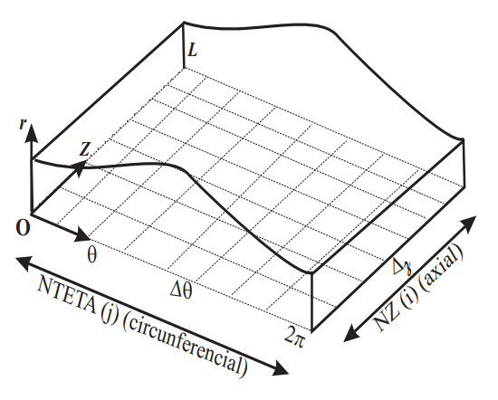
The discretized equation is given by

\[p_{i-1,j}\frac{(\mathbf{C_{2(i-1,j)}})}{\Delta z^{2}} + p_{i,j-1}\frac{(\mathbf{C_{1(i,j-1)}})}{\Delta\theta^{2}} - p_{i,j}\left(\frac{(\mathbf{C_{1(i,j)}} + \mathbf{C_{1(i,j-1)}})}{\Delta\theta^{2}} + \frac{(\mathbf{C_{2(i,j)}} + \mathbf{C_{2(i-1,j)}})}{\Delta z^{2}} \right) + p_{i,j+1} \frac{(\mathbf{C_{1(i,j)}})}{\Delta\theta^{2}} + p_{i+1,j}\frac{(\mathbf{C_{2(i,j)}})}{\Delta z^{2}} = \frac{1}{\Delta\theta}\left[\mathbf{C_{0W(i,j)}}-\mathbf{C_{0W(i,j-1)}}\right],\nonumber\]

with boundary conditions

\[p(z=0)=p(1,j)=P_{in}\]

\[p(z=L)=p(NZ,j)=P_{out}\]

\[p(\theta=0)=p(\theta=2\pi)=p(i,1)=p(i,N\theta)\]

Cavitation Condition

According to DOWNSON and TAYLOR (1979) [1], cavitation can be defined as the phenomenon that describes the discontinuity of a fluid due to the existence of gases or steam. This is a characteristic phenomenon in hydrodynamic bearings.

It is important to note that this change in pressure behavior due to cavitation does not necessarily start at the point of least thickness in the annular space. Several studies seek to establish the appropriate boundary conditions to describe the beginning of cavitation in the fluid. ISHIDA and YAMAMOTO (2012) [2] indicate that the condition of Gumbel is widely used because of its simplicity. Using the argument that lubricant evaporation and axial air flow from both ends can occur, the pressure in the region \(\pi < \theta < 2\pi\) is considered to be almost zero (that is, the atmospheric pressure ). \(p = 0 \) is then defined across the divergent region.

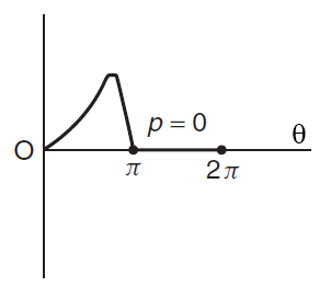
In addition, according to SANTOS (1995) [3], although it violates mass conservation, this condition presents acceptable errors in the global parameters of the bearing. For these reasons, the present study adopts the Gumbel boundary condition to describe the phenomenon of cavitation.

from ross.fluid_flow.fluid_flow_graphics import (
    plot_pressure_theta_cylindrical,
    plot_pressure_z,
    plot_pressure_theta,
    plot_pressure_surface,
)

my_fluid_flow.calculate_pressure_matrix_numerical()
fig1 = plot_pressure_z(my_fluid_flow, theta=int(my_fluid_flow.ntheta / 2))
fig1.show()
fig2 = plot_pressure_theta(my_fluid_flow, z=int(my_fluid_flow.nz / 2))
fig2.show()
fig3 = plot_pressure_theta_cylindrical(my_fluid_flow, z=int(my_fluid_flow.nz / 2))
fig3.show()
fig4 = plot_pressure_surface(my_fluid_flow)
fig4.show()

FORCES

The pressure field developes forces that acts on the rotor surface. According to SAN ANDRES (2010) [4] these forces are given by:

\[\begin{split} \begin{bmatrix} N \\ T \end{bmatrix} = R_i \int_{0}^{L} \int_{0}^{2\pi} p \begin{bmatrix} \cos{\theta}\\\sin{\theta} \end{bmatrix} d\theta dz\end{split}\]

As the pressure behavior is obtained numerically, the integrals above also need a numerical method to be solved. For this, the composite Simpson rule applied through the integrate.simps method of the library SciPy was chosen, by VIRTANEN et al. (2020) [5].

It is also possible to obtain the forces \( f_x \) and \( f_y \) in the Cartesian coordinate system:

\[\begin{split} f_x = T \cos{(\beta)} - N \sin{(\beta)} \\ f_y = T \sin{(\beta)} + N \cos{(\beta)}\end{split}\]

from ross.fluid_flow.fluid_flow_coefficients import calculate_oil_film_force

radial_force, tangential_force, force_x, force_y = calculate_oil_film_force(
    my_fluid_flow
)
print("N=", radial_force)
print("T=", tangential_force)
print("fx=", force_x)
print("fy=", force_y)

N= 245.11574757987194
T= 464.26637600572286
fx= 1.908338163048029e-06
fy= 524.9999977153587

EQUILIBRIUM POSITION

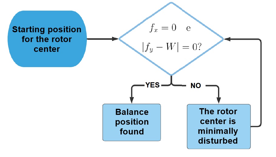
As indicated by SAN ANDRES (2010) [4], there is an equilibrium position in which the rotor center is stationary and the fluid film forces balance the external forces, in this case the rotor weight. This is expressed as:

\[f_{x_0} = 0\]

\[f_{y_0} = W \]

Knowing the external load \( W \), it is possible to reach the equilibrium position using an iterative method. Starting at an initial position, the residues between the forces at the current position and external forces are calculated. If the residue is greater than a defined tolerance, the position of the rotor is varied systematically, inside the fourth quadrant, until the desired tolerance is reached. In other words, a local minimum of the forces function is reached. The Python tool optimize.least_squares was used for this purpose. The method is shown in the image below.

from ross.fluid_flow.fluid_flow_coefficients import find_equilibrium_position

find_equilibrium_position(my_fluid_flow)
print("(xi,yi)=", "(", my_fluid_flow.xi, ",", my_fluid_flow.yi, ")")
radial_force, tangential_force, force_x, force_y = calculate_oil_film_force(
    my_fluid_flow
)
print("fx, fy=", force_x, ",", force_y)

(xi,yi)= ( 2.24665659581011e-05 , -1.186152916399651e-05 )
fx, fy= 6.35342044574827e-06 , 524.9999866137354

DYNAMIC COEFFICIENTS

According to SAN ANDRÉS (2010) [4], small disturbances around the equilibrium position allow us to express the fluid film forces as an expansion in Taylor series:

\[\begin{split}f_x = f_{x_0} + \dfrac{\partial f_x}{\partial x} \Delta x + \dfrac{\partial f_x}{\partial y} \Delta y + \dfrac{\partial f_x}{\partial \dot{x}} \Delta \dot{x} + \dfrac{\partial f_x}{\partial \dot{y}} \Delta \dot{y} \\ f_y = f_{y_0} + \dfrac{\partial f_y}{\partial x} \Delta x + \dfrac{\partial f_y}{\partial y} \Delta y + \dfrac{\partial f_y}{\partial \dot{x}} \Delta \dot{x} + \dfrac{\partial f_y}{\partial \dot{y}} \Delta \dot{y}\end{split}\]

From this expansion, the author also defines the stiffness coefficients \((k_{ij})\), damping \((c_{ij})\) as:

\[ k_{ij}=-\dfrac{\partial f_i}{\partial j}\text{;} \quad \quad c_{ij}=-\dfrac{\partial f_i}{\partial \dot{j}}\text{;} \quad \quad i,j \in x,y\]

The procedure to calculate these coeficients is divided in three steps. First, two perturbations along the \(x\) and \(y\) directions are considered in the calculation of the velocity of any point \(A\) in the rotor surface. This is expressed as

\[v_{tot} = v_{rot} + v_p\]

where \(v_{rot}\) is the velocity of the point due to the rotation and \(v_{p}\) is the velocity acquired by a disturbance along each direction. These perturbation are considered of the type

\[\begin{split}(v_p)_x = \omega_p x_p \cos{(\omega_p t)}e_x \longrightarrow \text{for a perturbation along the $x$ direction} \\ (v_p)_y = \omega_p y_p \cos{(\omega_p t)}e_y \longrightarrow \text{for a perturbation along the $y$ direction},\end{split}\]

where \(e_x\) and \(e_y\) are unit vectors in cartesian coordinates.

Combination of the two last equations, in cylindrical coordinates, gives the following velocity along each axis:

\[\begin{split}(v_{tot})_x = \underset{v(R_\theta)_x}{\underbrace{\left(\omega \dfrac{\partial R_{\theta}}{\partial \theta} + \omega_p x_p \cos{(\omega_p t)\cos{(\theta)}}\right)}} e_r + \underset{w(R_\theta)_x}{\underbrace{\left(\omega R_{\theta} - \omega_p x_p \cos{(\omega_p t)}\sin{(\theta)} \right)}} e_{\theta} \\ (v_{tot})_y = \underset{v(R_\theta)_y}{\underbrace{\left(\omega \dfrac{\partial R_{\theta}}{\partial \theta} + \omega_p y_p \cos{(\omega_p t)\sin{(\theta)}}\right)}} e_r + \underset{w(R_\theta)_y}{\underbrace{\left(\omega R_{\theta} - \omega_p y_p \cos{(\omega_p t)}\cos{(\theta)} \right)}} e_{\theta}\end{split}\]

The second step is to substitute the radial speeds (\(v(R_\theta)_x\) and \(v(R_\theta)_y\)), and tangential speeds(\(w(R_\theta)_x\) and \(w(R_\theta)_y\)) in the continuity equation, previously calculated for a fixed position. Thus, when the rotor is rotating and its center is being perturbed along horizontal and vertical directions, the new \(C_0\) coefficient of the continuity equation is

\[\begin{split}(C_0)_x = C_0 + \left[R_{\theta} \omega_p x_p \cos{(\omega_p t)} \sin{(\theta)}\right] \\ (C_0)_y = C_0 + \left[R_{\theta} \omega_p y_p \cos{(\omega_p t)} \cos{(\theta)}\right]\end{split}\]

This new coefficient ensures that the fluid film forces are calculated for a rotor with a fixed rotation \(\omega\) and with a center moving along a horizontal or vertical direction with a fixed frequency \(\omega_p\).

The final step is to calculate the forces, along both the horizontal and vertical directions, for each perturbation. This sets the following four equations:

\[\begin{split}\left( f_x[t] \right)_x = f_{x_0} + k_{xx}\Delta x[t] + c_{xx}\Delta \dot{x}[t]\text{,} \\ \left( f_y[t] \right)_x = f_{y_0} + k_{yx}\Delta x[t] + c_{yx}\Delta \dot{x}[t]\text{,} \\ \left( f_x[t] \right)_y = f_{x_0} + k_{xy}\Delta y[t] + c_{xy}\Delta \dot{y}[t]\text{,} \\ \left( f_y[t] \right)_y = f_{y_0} + k_{yy}\Delta y[t] + c_{yy}\Delta \dot{y}[t] \end{split}\]

where the only unkowns are the eight coefficients. In matrix form, this equation is expressed as follows

\[\begin{split}\mathbf{A}_x \begin{bmatrix} k_{xx} & k_{yx}\\ c_{xx} & c_{yx} \end{bmatrix} = \mathbf{F}_x \quad \quad \text{e} \quad \quad \mathbf{A}_y \begin{bmatrix} k_{xy} & k_{yy}\\ c_{xy} & c_{yy} \end{bmatrix} = \mathbf{F}_y\end{split}\]

The coefficients are obtained by using the Moore Penrose inverse and solving for each set of coefficients:

\[\begin{split}\begin{bmatrix} k_{xx} & k_{yx}\\ c_{xx} & c_{yx} \end{bmatrix} = \left( \mathbf{A}_{x}^{T} \mathbf{A}_{x}\right)^{-1} \mathbf{A}_{x}^{T} \mathbf{F}_x \quad \quad \text{e} \quad \quad \begin{bmatrix} k_{xy} & k_{yy}\\ c_{xy} & c_{yy} \end{bmatrix} = \left( \mathbf{A}_{y}^{T} \mathbf{A}_{y}\right)^{-1} \mathbf{A}_{y}^{T}\mathbf{F}_y\end{split}\]

from ross.fluid_flow.fluid_flow_coefficients import (
    calculate_stiffness_and_damping_coefficients,
)

K, C = calculate_stiffness_and_damping_coefficients(my_fluid_flow)
kxx, kxy, kyx, kyy = K[0], K[1], K[2], K[3]
cxx, cxy, cyx, cyy = C[0], C[1], C[2], C[3]
print("Stiffness coefficients:")
print("kxx, kxy, kyx, kyy = ", kxx, kxy, kyx, kyy)
print("Damping coefficients:")
print("cxx, cxy, cyx, cyy", cxx, cxy, cyx, cyy)

Stiffness coefficients:
kxx, kxy, kyx, kyy =  15121431.698482102 15384601.661070675 -25817662.364928093 13631622.300446654
Damping coefficients:
cxx, cxy, cyx, cyy 270679.3080703647 -142944.89893464962 -27092.083591982722 312029.25118641555

Based on MOTA (2020), where is the complete theory used by FluidFlow:

Mota, J. A.; Estudo da teoria de lubrificação com parametrização diferenciada da geometria e aplicações em mancais hidrodinâmicos. Dissertação de Mestrado - Programa de Pós-Graduação em Informática, Universidade Federal do Rio de Janeiro, Rio de Janeiro, 2020

REFERENCES CITED IN THE TEXT

[1] DOWSON, D.; TAYLOR, C. Cavitation in bearings. Annual Review of Fluid Mechanics, [S.l.], v. 11, n. 1, p. 35–65, 1979.

[2] ISHIDA, Y.; YAMAMOTO, T. Flow-Induced Vibrations. In: Linear and nonlinear rotordynamics. Weinheim: Wiley Online Library, 2012. p. 235–261.

[3] SANTOS, E. S. ** Carregamento dinamico de mancais radiais com cavitaçãodo filme de óleo**. Dissertação de Mestrado — Centro Tecnológico, Universidade Federal de Santa Catarina, Santa Catarina, 1995.

[4] SAN ANDRES, L. Experimental Identification of Bearing Force Coefficients, Notes 1 5 Acesso em 08/02/2020, http://oaktrust.library.tamu.edu/handle/1969.1/93199.

[5] VIRTANEN, P. et al. SciPy 1.0: fundamental algorithms for scientific computing inpython. Nature Methods, [S.l.], v. 17, p. 261–272, 2020.