Release notes

Release notes#

Version 3.1.0#

ROSS 3.1.0 adds a three-phase induction motor model that drives the rotor time response (MotorElement and Rotor.run_with_motor), a mesh convergence analysis with shaft refinement methods (Rotor.run_mesh_convergence, Rotor.refine and Rotor.refine_mesh), gear mesh damping for MultiRotor, time windows in the time-response plots, a helper that builds speed ranges from their end points, and a 3-D rotor view and new modeling tools in the graphical interface.

Although this is a minor release, it breaks code written for 3.0. CoAxialRotor, coaxrotor_example, Rotor.convergence and ConvergenceResults were removed and MultiRotor.K_coupling was renamed coupling_matrix, all without a deprecation period. The default mesh damping of backlash models changed from 0.07 to 0, the new motor_element parameter of Rotor moves min_w and the following parameters one position to the right, and the frequency-response plots read off-diagonal pairs as the response at out to a force at inp, the transpose of what they plotted in 3.0. ROSS 3.1 supports Python 3.13 to 3.15; Python 3.12 is no longer supported. Read API Changes below before upgrading.

The following enhancements and bug fixes were implemented for this release:

Enhancements#

Three-Phase Induction Motor: `MotorElement` and `run_with_motor`#

The new ross.motors subpackage models a three-phase induction motor. Contributed by Jessica Guarato and Bruno Zambolini Vicente (#1296):

MotorElement(n, power_rated, voltage_rated, speed_rated, stator_resistance, rotor_resistance, stator_reactance, rotor_reactance, mutual_reactance, Ip_motor, ...) is the motor at node n; rs.motor_example() returns one. The motor can be simulated on its own with run_direct_on_line() (direct-on-line start, with optional grid harmonics and voltage unbalance), run_with_inverter_vf() (V/f inverter) or run_with_inverter_foc() (field-oriented-control inverter). The time loops are fourth-order Runge-Kutta steps compiled with numba. The results are a MotorResponseResults, with plot_torque(), plot_speed(), plot_phase_currents(), plot_phase_voltages() and plot_line_voltages(), and PhaseResults plots a phase signal and its DFFT. Both classes are defined in ross.motors.results and exported from ross, like the other results classes (#1445).
A rotor carries at most one motor, given as Rotor(..., motor_element=motor) or added with rotor.add_elements([motor]), which replaces an existing motor. The motor has zero mass, stiffness, damping and gyroscopic matrices, so it does not change the rotor matrices. It is listed in Rotor.df, drawn by plot_rotor, kept and renumbered by add_nodes, refine and refine_mesh (#1439) and saved and loaded with the rotor. Rotor.concatenate keeps the motor of the last rotor that has one. A MultiRotor takes the motor of its driving or its driven rotor; when both carry one, MultiRotor raises Warning (an exception).
Rotor.run_with_motor(t, node, unbalance_magnitude, unbalance_phase, drive_mode, ...) simulates the motor with drive_mode "DOL", "VFD_VF" or "VFD_FOC", applies the electric torque minus the load torque to the torsional degree of freedom of the motor node, computes the unbalance force from the motor speed history and integrates the rotor with the Newmark method, adding the torque-dependent stiffness ShaftElement.Ktq() * torque of the shaft elements at the motor node. With the default steady_state=True only the last third of the interval after load_torque_entrance_time is integrated. It returns a TimeResponseResults whose motor_results attribute holds the motor simulation.
Also added: ShaftElement.Ktq(), the torque stiffness matrix per unit torque, which ShaftElement.K() now uses for its torque term (the matrix values are unchanged); Ktq and torque keyword arguments of the time integration with a speed array; ross.units.format_unit(), which formats a unit as an axis label ("N*m" becomes "N⋅m"); ross.utils.downsample_figure() and ross.utils.limit_data_range(); and the unit cv (metric horsepower).
The new tutorial tutorial_motor (“Tutorial - Three-Phase Induction Motor”) is in the user guide.

Gear Mesh Damping for `MultiRotor`#

MultiRotor accepts mesh_damping_ratio (dimensionless, a float or a quantity such as Q_(7, "percent"), default 0.0). The mesh damping coefficient $c_m = 2 \zeta \sqrt{k_m M_{eq}}$ (Yi et al., 2019) multiplies the same coupling matrix as the mesh stiffness. Without backlash it is added to MultiRotor.C() by the new MultiRotor.C_mesh(), so modal, Campbell, frequency, forced and time responses include it; with backlash the same ratio enters the nonlinear contact force. When the mesh stiffness varies in time, $c_m$ follows the stiffness of the current step. The equivalent mass $M_{eq}$ is the new Mesh.M_eq, computed from the polar inertias and base radii of the gears, so $\zeta$ is the damping ratio of the torsional mesh mode. The MultiRotor tutorial describes the model. Contributed by Murillo Alvaro Borges de Sousa (#1427).

Time Windows in Time-Response Plots#

TimeResponseResults.plot_1d, plot_2d and plot_3d accept the keyword options t_initial and t_final, which plot a window of the stored response without running the simulation again, and one_revolution=True, which plots one shaft revolution: the last one, or the one that starts at t_initial or ends at t_final. Contributed by Murillo Alvaro Borges de Sousa (#1416, issue #1415):

Plain numbers are read in the time_units of plot_1d and in seconds by plot_2d and plot_3d; quantities keep their units. A window outside the stored interval, t_initial >= t_final or a window with fewer than 10 samples (ross.results.MIN_WINDOW_SAMPLES) raise ValueError; the message for a short window gives the time step that would be enough. With one_revolution=True this needs a time step of at most 2 * pi / (9 * speed) s (#1443). A plain window needs both t_initial and t_final, and one_revolution=True takes at most one of them (ValueError otherwise).
The revolution length is computed from the speed the results now store (TimeResponseResults.speed); a speed that varies along the response is integrated. one_revolution=True raises ValueError when the results hold no speed.
A windowed plot_1d sets the x-axis range to the window, and windowed plot_2d and plot_3d mark the initial and final points.
TimeResponseResults, AmbTimeResponseResults and BacklashResults take and store the run speed (speed=None), and data_time_response accepts t and yout arrays in place of the stored ones.

Speed Ranges from End Points#

ross.utils.speed_range_from_endpoints(speed_start, speed_stop, num_points=None, points_factor=20) returns an evenly spaced speed array in rad/s for run_campbell, run_freq_response and run_unbalance_response. Each end point can be given in its own unit (Q_(0, "Hz"), Q_(3600, "RPM")). Without num_points the count is ceil(points_factor * sqrt(span)), with the span in rad/s, limited to [20, 2000], so a narrow range gets a finer step than a wide one; about 4 is enough as points_factor for a Campbell diagram. It raises ValueError when speed_stop <= speed_start or num_points < 2. The three run_* docstrings point to it; their signatures are unchanged. The function is in ross.utils and is not exported from the top-level ross namespace. Contributed by Vinicius Vianna (#1414).

Graphical Interface#

The graphical interface (ross-interface) gained the following, contributed by Leonardo Cabral:

3-D rotor view. The modeling screen shows a 3-D view beside the 2-D ROSS figure, drawn from a scene the server builds from the assembled rotor. A right-button menu splits, discretizes, edits, copies, hides, adds and deletes elements; the view shows node numbers and dimensions, has a measuring tape, a legend that hides categories and an optional motor bench. three.js r186 is vendored under ross/interface/frontend/vendor/three/ and loaded the first time the view opens (#1429).
Discretization and filters. Shafts can be discretized by length-to-diameter ratio (API RP 684), into a number of parts, or by Rotor.run_mesh_convergence (refused for rotors coupled by gears), and the element list can be filtered by material, model, node, tag or field value (#1429).
Geometry and probes. Disks and gears can be entered by their dimensions (DiskElement.from_geometry, GearElement.from_geometry). A new probe category places radial and axial probes on the model; analysis probe tables and the frequency-response output can name these probes, and their tags reach the chart legends (#1429).
Modeling tools. Rotor concatenation (Rotor.concatenate) and shaft splitting (Rotor.add_nodes) have their own dialogs; Ctrl+Z / Ctrl+Y undo and redo; several elements can be selected and copied or deleted together (#1419).
Rotor figure and layout. The screen keeps the geometry of the figure ROSS returns and applies a declared vertical exaggeration; the layout has a minimum width instead of reflowing in narrow windows (#1419).
Projects. Project files are loaded as written, so a saved MultiRotor reopens as one instead of as an empty rotor, and files with old Portuguese key names still load. The MultiRotor dialog shows where each rotor’s gears are, fills the coupled nodes when only one choice exists and builds the MultiRotor on the server before saving, so a ROSS error appears while the fields are still on screen (#1419).
Materials. Spaces in material names become underscores, because rs.Material refuses spaces, and an element that names a material the project does not have is refused with “This rotor has no material by that name” (HTTP 400); before, it silently got the first material (#1419).
Analyses. The frequency-response and unbalance forms have a Steps field (default 50; it was fixed at 50), and the Campbell, clearance, frequency-response and unbalance sweeps refuse fewer than 2 steps. The speed fields are number fields without bounds instead of sliders. An empty nodes field of the modal orbit plot draws every node, and an unknown node is refused with the list of the rotor’s nodes. Exceptions that ROSS raises on purpose return HTTP 400 with their message alone; before, those other than ValueError were a 500 shown as “Unexpected error (<type>): <message>” (#1419).

The Advanced section of the MultiRotor form has a Mesh Damping Ratio [-] field (default 0.0), passed to rs.MultiRotor as mesh_damping_ratio, written into exported scripts and kept in the project file. An empty field, or a project saved without it, leaves the argument out, so the library default applies. A negative ratio is refused with “The mesh damping ratio must be zero or positive” (#1444).

Bug Fixes#

Fix Double Unit Conversion in `plot_1d` and `plot_dfft`#

TimeResponseResults.plot_1d() and plot_dfft() converted to displacement_units the response that data_time_response() had already converted, so any unit other than "m" scaled the plot by the conversion factor a second time (1e3 too large in "mm", 1e6 in "um"). Plots in "m" are unchanged. Contributed by Gabriel Sabino (#1418, issue #1417).

Fix NaN AMB Time Response with scipy 1.18 and Later#

With scipy 1.18 and later, run_time_response on AMB rotors whose controllers are high-order transfer functions (for example rotor_example_amb_complex_controllers()) returned NaN for every output: the companion-form realization of the controllers gave a closed-loop matrix with a 1-norm around 1e26, and the matrix exponential inside scipy.signal.lsim overflowed. AmbTimeResponse.build_matrices (ross.bearings.magnetic.amb_time_response) now balances [[A_cl, B_cl], [C_cl, 0]] with scipy.linalg.matrix_balance, which rescales only the state; the new attribute state_scaling holds the factors (physical state = state_scaling * z), the initial condition is converted, and inputs and outputs keep their physical units. Contributed by Jessica Guarato (#1422, issue #1421).

Fix `MultiRotor` Rebuilds Dropping the Mesh Settings#

MultiRotor.add_nodes and add_elements rebuilt the model without its backlash settings and rebuilt the square-wave stiffness from the mesh attributes. The rebuilt model now keeps the backlash and square_varying_stiffness dictionaries and the gear_mesh_stiffness given to the constructor (#1427).

Fix `ModalResults.plot_orbit` Without Nodes#

ModalResults.plot_orbit(mode) with the default nodes=None returned an empty figure. It now plots the orbit of every node of the mode shape (#1419).

Fix Frequency-Response Plots Reading the Transposed Entry#

run_freq_response stores $H = Z^{-1}$, so freq_resp[out, inp, i] is the response at out to a unit force at inp. FrequencyResponseResults.plot_magnitude, plot_phase, plot_polar_bode (and so plot) and ST_Rotor.run_freq_response read freq_resp[inp, out]. On a gyroscopic rotor at speed the cross x/y pairs had the phase off by $\pi$, and with cross-coupled bearings (kxy != -kyx) magnitude and phase were wrong on every off-diagonal pair. They now read freq_resp[out, inp]; the stored array is unchanged and diagonal pairs plot as before. The probe outputs of the interface frequency-response analysis, and the probe_output function written into exported scripts, projected the force axis to match the old reading, which mirrored a radial probe at angle $a$ to $-a$. They now project the response axis (#1441, #1449).

Fix `add_nodes` and `refine_mesh` Moving AMB Sensors and Disk Nodes#

Rotor.add_nodes, and through it refine_mesh, renumbered the shaft but left the sensor_node of magnetic bearings and the n_l / n_r of disks at the old numbers, so a collocated AMB became non-collocated and AMB results were wrong. They now use the renumbering of Rotor.refine. add_nodes also renumbers the motor’s n_l / n_r with its n, and refine keeps the motor, which it dropped (#1439).

Fix `check_units` with pint 0.26.2#

pint 0.26.2 parses a string magnitude as an expression and raises AssertionError for Q_("major", "rad"). check_units relied on a TypeError there to return option strings unchanged, so calls such as Probe(3, "major") and run_campbell(frequency_type="wd") failed. check_units now returns str arguments without converting them, and Probe.get_label checks for a string angle (#1438).

Fix the Mayes and Gasch Crack Models with pandas 3.1#

Crack read the Papadopoulos compliance table with pd.eval on a whole column, which pandas 3.1 refuses, so crack_model="Mayes" and "Gasch" failed. The table is now parsed with json.loads; the coefficients are unchanged (#1456).

Fix the Version Warning of `compressor_example`#

rs.compressor_example() reads a TOML file shipped with ROSS and emitted the UserWarning “File was created with ROSS 3.0.0.dev0, but current version is …” at every call once the minor version changed. It now builds the rotor without the version check; Rotor.load warns for other files as before (#1440).

Documentation and Agent Tooling#

Documentation#

Fourteen notebooks whose stored figures still showed the frame used before the right-handed frame of 3.0.0 were re-executed: the getting-started overview, the modeling, analyses and MultiRotor tutorials, and examples 5, 16, 22, 24, 28, 29, 30 and 31. Example 31 runs again (frequencies=8 moved from CampbellResults.plot to run_campbell, and run_modal asks for num_modes=16). docs/user_guide/rotor2.toml was regenerated in the 3.x save format, and the README lost its emojis and has the codecov badge in Markdown and the corrected name of the Federal University of Uberlândia (#1412).
tutorial_analyses_part_2 and the run_time_response docstring describe t_initial, t_final and one_revolution (#1416), and tutorial_multirotor describes the mesh damping model, with Visnadi (2022) added to the references (#1427).
The API reference lists Rotor.run_mesh_convergence, Rotor.refine and MeshConvergenceResults instead of ConvergenceResults (#1420).
CoAxialRotor and coaxrotor_example were dropped from the API reference, and example 25 is now titled “Overhung Rotor on Flexible Supports”; it is Friswell’s Example 6.8.1 and never used CoAxialRotor (#1434).
ross/interface/README_INTERFACE.md describes the 3-D view (#1429).
The API reference lists MotorElement, motor_example, Rotor.run_with_motor, Rotor.run_amb_non_collocation, Rotor.refine_mesh, MotorResponseResults, PhaseResults, AmbNonCollocationResults, SourceAC, InverterVF, InverterFOC (in a new “Motor Drives” section) and ross.utils.speed_range_from_endpoints; the entries rotor_amb_example and concatenate_rotor, which name nothing in ross, gave way to the three rotor_example_amb_* functions. The docstrings of run_with_motor, run_direct_on_line, run_harmonic_balance_response, run_level1, run_misalignment and MotorResponseResults.sample_at render without docutils errors. The MotorElement docstring and tutorial_motor state that the constructor’s voltage_net and frequency_net do not set the direct-on-line supply and that the steady_state=True window starts from rest (#1445).
tutorial_stochastic, tutorial_motor, tutorial_bearings_part_3 and tutorial_modeling_part_1 run without errors or side effects: the stochastic unbalance response draws var_size samples and its sweeps start at 1 rad/s, the figures use the notebook renderer instead of renderer="svg" (which needs kaleido), and the material example saves and removes my_steel instead of overwriting the packaged Steel entry. example_2, tutorial_units, tutorial_bearings_part_1, tutorial_bearings_part_2 and tutorial_seals were executed again, and the tqdm IProgress not found stderr output was removed from 18 notebooks (#1446). The stored version warning of compressor_example() was removed from tutorial_analyses_part_1 and tutorial_analyses_part_2 (#1440).
The run_time_response doctest and the one-revolution example of tutorial_analyses_part_2 use a time step that puts about 50 samples in each revolution (#1443).
The installation page, AGENTS.md and ross/interface/README_INTERFACE.md give Python 3.13 as the oldest supported version, and the installation page describes the downsample extra (#1447).

Agent Tooling#

AGENTS.md is the only instruction file for coding agents; CLAUDE.md was removed and its content moved there. It holds the usage reference (analysis methods with their results classes, plots and recipes, example rotors and units) and the development rules: the five criteria a contribution must meet, scope, architecture, tests, writing, pull requests and reviewing, including that agents never post to GitHub without explicit approval. The new .github/PULL_REQUEST_TEMPLATE.md has the sections Summary, Scope, Design decisions for review, API changes, Evidence, Changes to existing tests or reference data, Documentation and Where to look, and CONTRIBUTING.md points to it and to AGENTS.md (#1432).
Two agent skills for contributors and reviewers: ross-pr-create (.agents/skills/ross-pr-create/) checks a change against AGENTS.md, runs the checks and drafts the PR text from the template; ross-pr-review (.agents/skills/ross-pr-review/) reviews a pull request, runs correctness probes on its head and base and can write an HTML report, and posts nothing to GitHub until the person who asked approves. Both use the new tools/pr_facts.py (--base, --head, --json), which compares two revisions with git and ast only, without running the PR code. .claude/skills/ links to both skills, CI runs pytest tools/tests, and ruff also checks tools/ and .agents/. The ross package is unchanged (#1433).
The review report of ross-pr-review turns its page background dark in dark mode, and a pipe escaped as \| or written inside a code span stays in its table cell (#1436).
The agent skill has a motor recipe, following tutorial_motor, and SKILL.md indexes every Rotor.run_* method, with help(...) rows for run_harmonic_balance_response, run_amb_sensitivity and run_amb_non_collocation, which have no recipe yet. The time_response recipe shows the plot windows, and the Campbell, unbalance and frequency response recipes use speed_range_from_endpoints. AGENTS.md lists run_with_motor, motor_example and ross/motors/ (#1445). The frequency_response recipe gives freq_resp[out, inp, :] as the plotted entry (#1441).

Release Process#

The Release workflow (publish-to-pypi.yml) runs tools/check_release_version.py between the build and the upload. It stops the release unless the tag is v followed by the canonical version of every built wheel and sdist, so a tag pushed before the version bump no longer uploads a .dev0 package; CONTRIBUTING.md describes the check (#1448).
CI tests Python 3.13, 3.14 and 3.15, and the release is built on 3.13 (#1447).

API Changes#

Removed classes, methods and attributes#

None of these has a deprecated alias: the old name raises AttributeError (ImportError for from ross import ...).

Removed	Replacement
`CoAxialRotor`	none; stay on 3.0.x (where only part of the analyses worked, see #1430) until coaxial support returns
`coaxrotor_example()`	none
`Rotor.convergence(n_eigval, err_max)`	`Rotor.run_mesh_convergence(rtol, frequencies, ...)`
`MultiRotor.convergence` (inherited)	none; `run_mesh_convergence` and `refine` raise `NotImplementedError` on `MultiRotor`
`Rotor.error_arr`	`MeshConvergenceResults.errors` / `.error`
`ConvergenceResults`	`MeshConvergenceResults`
`MultiRotor.K_coupling`	`MultiRotor.coupling_matrix` (same values)

CoAxialRotor was removed because about half of the analyses failed on a coaxial rotor in 3.0 (among them run_static, run_ucs, run_level1, convergence and add_nodes), both shafts ran at one speed, and saved coaxial rotors could not be loaded (#1434, issue #1430). The rework in #1423 was closed, and coaxial support may return in a later release. MultiRotor is unchanged.

Rotor.convergence (#1420) checked one eigenvalue, doubled the number of elements at every step and replaced the rotor’s contents in place. run_mesh_convergence checks the lowest frequencies natural frequencies, so n_eigval=k is covered by frequencies=k + 1. err_max (default 1e-2) bounded the change between two successive doublings; rtol (default 1e-3) bounds the error against a converged reference. On a MultiRotor, convergence rebuilt the model as a plain Rotor without the gear mesh. The refined rotor is results.rotor, and the rotor the method is called on is not modified. ConvergenceResults (el_num, eigv_arr, error_arr) gave way to MeshConvergenceResults (elements, wn, wn_reference, errors, error, …).

K_coupling was renamed because the matrix now multiplies both the mesh stiffness and the mesh damping (#1427).

Changed signatures#

Rotor.__init__ has motor_element=None as its fifth parameter, after point_mass_elements. min_w, max_w, rated_w, modal_damping_ratio, default_damping_ratio, alpha, beta and tag each move one position to the right, so a call that passes min_w or a later argument by position now binds it to motor_element. Pass those arguments by keyword (#1296).
ross.multi_rotor.mesh.Backlash.__init__ has a new required parameter M_eq between damping_ratio and module, which Mesh now passes. Only code that builds Backlash directly is affected (#1427).
Parameters added at the end, so positional calls keep working: MultiRotor(..., mesh_damping_ratio=0.0) (#1427); TimeResponseResults, AmbTimeResponseResults and BacklashResults take speed=None, and data_time_response takes t=None and yout=None (#1416).
Shape.plot_orbit(nodes, fig=None) became Shape.plot_orbit(nodes=None, fig=None); with nodes=None it plots every node (#1419).

Changed defaults and behavior#

Mesh damping of backlash models. The default damping_ratio of Mesh changed from 0.07 to 0.0, and MultiRotor now passes its mesh_damping_ratio (default 0.0) to it. In 3.0 MultiRotor passed no ratio, so a backlash model built with default arguments used 0.07; in 3.1 it has no mesh damping, and its time responses change (the transmission error and the mesh force). Pass mesh_damping_ratio=0.07 to MultiRotor (or damping_ratio=0.07 to Mesh) to reproduce 3.0 results. Models without backlash had no mesh damping in 3.0 and have none with the default (#1427). The interface’s MultiRotor form has a field for the ratio (#1444).
MultiRotor.add_nodes and add_elements rebuild the model with the gear_mesh_stiffness given to the constructor, so a value assigned to mesh.stiffness afterwards, or left there by a time response with update_mesh_stiffness=True, is not carried over (#1427).
Rotor.disk_elements and Rotor.point_mass_elements are sorted by node number; before, they kept the order they were given in (#1296).
Rotor.add_elements accepts a MotorElement, which replaces the rotor’s motor (#1296). Other objects that are not supported elements still raise ValueError("<obj> is not a valid element."), and MultiRotor.add_elements now raises the same ValueError for them instead of AttributeError (#1442).
Frequency-response plots. For inp != out, FrequencyResponseResults.plot_magnitude, plot_phase, plot_polar_bode and plot plot freq_resp[out, inp], the response at out to a unit force at inp, and ST_Rotor.run_freq_response stores those samples; in 3.0 they used freq_resp[inp, out]. Off-diagonal plots change wherever $H$ is not symmetric (gyroscopic rotors at speed, cross-coupled or anisotropic bearings). Scripts that swapped inp and out to get the response at out now get the transposed entry and must swap them back (see Bug Fixes, #1441).
Functions decorated with check_units return str arguments unchanged. A numeric string such as "3" given for a unit argument stays a string; pint converted it to the number 3 before (#1438).
Rotor.add_nodes ignores repeated positions (3.0 raised ZeroDivisionError) and no longer sorts the caller’s new_nodes_pos list in place. For layered shafts, the tags of the shaft elements of the returned rotor follow the order of the pieces of each original element, as in refine, instead of their position; geometry and numbering are unchanged (#1439).
ross.utils.downsample_figure keeps at most max(n_out, 4) points of each trace; n_out below 4 is raised to 4 (#1447).
BacklashResults.PARAMS: the "units" key of every entry is now "unit", and the unit of contact_ratio is "dimensionless" instead of "--" (#1296).
TimeResponseResults.plot_dfft(frequency_range=...) raises ValueError when the range contains no DFFT points; before, the trace was empty (#1296).
With displacement_units other than "m", plot_1d and plot_dfft no longer apply the unit conversion twice, so their values differ from 3.0 by the conversion factor (see Bug Fixes, #1418).
The progress messages “Running direct method” and “Running with model reduction: …” of the time integration (run_time_response, run_crack, run_rubbing, run_misalignment) end with a carriage return instead of a newline, so the next output overwrites them (#1296).
AmbTimeResponse.A_cl, B_cl and C_cl are stored in the balanced coordinates after build_matrices, in which the physical state is state_scaling * z. D_cl and the outputs are unchanged (#1422).

Saved files#

A rotor with a motor is saved with a MotorElement section, which ROSS 3.0 cannot read. Rotor files without a motor are unchanged (#1296).
TimeResponseResults, AmbTimeResponseResults and BacklashResults files store the run speed. Files saved by 3.0 load in 3.1 with speed=None (so one_revolution=True is not available for them); files saved by 3.1 from run_time_response store the speed and fail to load in 3.0 with TypeError (#1416).
ConvergenceResults files can no longer be loaded; MeshConvergenceResults has its own format, which stores the refined rotor (#1420).
Coaxial rotor files did not load in 3.0 either, and still do not (#1434).

Dependencies#

Python. requires-python is >=3.13: ROSS 3.1 supports Python 3.13, 3.14 and 3.15, and Python 3.12 is dropped, following the SPEC 0 support window. Stay on 3.0.x for Python 3.12 (#1447).
Floors. plotly>=5.15 (was 5.11) and pint>=0.24.4 (was 0.18); the older versions do not work with the numpy 2.2 floor. The other minimum versions are those of 3.0.0 (#1447).
tsdownsample (optional). downsample_figure thins the traces of the motor result plots (#1296). It uses the MinMaxLTTB algorithm of tsdownsample when that package is installed, with the new extra pip install "ross-rotordynamics[downsample]" (tsdownsample>=0.1.5, which has no wheels for Python 3.15); otherwise it falls back to a min-max decimation in numpy that keeps the lowest and highest sample of each interval and the first and last samples. tsdownsample is imported when downsample_figure is called, and the private module attribute ross.utils._downsampler was removed (#1447).
The interface vendors three.js r186 (MIT license, about 2.1 MB) inside the package, with no new Python dependency (#1429).

Interface Project Files, Scripts and Routes#

The frontend no longer publishes its functions on window, and buttons dispatch data-action attributes instead of inline HTML handlers; scripts that called those globals stop working (#1419).
A coupling with a blank n is numbered by its position in the list, and values such as 1_0 or 0x10 count as blank (#1419).
Project files have a probes category, disks and gears can have the element type Geometry, and any element can carry a shape3d field used only by the 3-D view; files without them load with empty values (#1429). Project files can carry multi_params.mesh_damping_ratio; files without it load and build as before (#1444).
The probe_output function written into exported scripts returns arrays of shape (1, ndof, nfreq) instead of (ndof, 1, nfreq): the probe is output 0 (#1441).
Exported Python scripts write step counts as integer literals and refuse non-numeric ones, use the Steps field for the unbalance sweep, write material names with underscores (#1419), and build disks from a list of (constructor, kwargs) pairs so DiskElement.from_geometry can appear (#1429).
The /build_rotor route takes an optional figure field (default true; false skips the 2-D figure) and returns the 3-D scene. New routes: /api/rotor/concatenate and /api/rotor/split_shaft (#1419), /api/rotor/mesh_shafts and /api/units/convert (#1429).

Known Issues#

The motor coupling of Rotor.run_with_motor (#1296) has the following open problems in 3.1.0. The stand-alone motor analyses of MotorElement match the steady-state equivalent circuit and are not affected by the first two.

Speed history. The motor speed is integrated with Ip_motor + Ip_load only, not with the inertia of the rotor model, and the net torque is also applied to the torsional degree of freedom of the motor node. With the default Ip_load=0 the start-up is too fast (18.8 times on the rotor of the tutorial), so run-ups through a critical speed are wrong. The torsional displacements drift without bound; the lateral response is not affected by the drift.
Default steady-state window. With steady_state=True the integration starts from rest inside the window, and the free vibration has not decayed when it ends: unbalance amplitudes read 19 % to more than 100 % above the forced response, depending on the damping. Use steady_state=False and discard the start of the response.
Save and load. MotorResponseResults and PhaseResults fail to load after save, and the motor_results attribute of the results of run_with_motor is not saved.
Force array. run_with_motor adds the unbalance force and the torque to the F array it is given, in place. Pass a copy when calling it more than once with the same array.
Supply settings. The voltage_net and frequency_net given to the MotorElement constructor are ignored by run_direct_on_line; pass them to the run_* call. load_torque_entrance_time and viscosity_coeff accept only floats, not Q_ values (viscosity_coeff is a rotational friction coefficient in N·m·s/rad, not a viscosity), and stator_reactance and rotor_reactance are leakage reactances.
Motor on a MultiRotor. A motor on the driven rotor receives the speed of the driving rotor.

These will be addressed in a later release.

Contributors#

This release includes contributions from: @jguarato, @bgglzv, @viniciuserrav, @murilloabs, @gsabinoo, @leonardocabr, @raphaeltimbo

Version 3.0.0#

ROSS 3.0.0 is a major release. Beyond the library API, it adds two new ways of working with ROSS:

A graphical interface. pip install "ross-rotordynamics[interface]" followed by ross-interface opens a local web application that builds rotors from forms, draws them, runs every analysis in its own dashboard and exports the model as a ready-to-run Python script. Every GitHub release also carries a Windows bundle that needs no Python. See Graphical Interface below.
An agent skill for AI coding assistants. ross-install-skill installs the ROSS cookbook as an Agent Skill into Claude Code, GitHub Copilot, Cursor and Codex, so an AI coding agent knows how to build rotors and run analyses with the current API. See Agent Skill for AI Coding Assistants below.

The library itself gained a thermo-elasto-hydro-dynamic engine for journal bearings, coefficient tables that decouple the rotor speed from the excitation frequency, an API 617 clearance analysis, closed-loop time response and sensor non-collocation analysis for active magnetic bearings, a gear backlash model, right-handed plot frames and a dark Plotly template. Since parameter names and conventions changed without deprecation shims, the ross_2to3 tool converts ROSS 2 rotor files, scripts and notebooks to the new API.

The following enhancements and bug fixes were implemented for this release:

Enhancements#

Graphical Interface#

ROSS 3 ships a graphical interface: a local web application (Flask backend, JavaScript frontend) that builds rotors from forms derived from the library’s own classes, draws them, runs the analyses and exports the model as a Python script, contributed by Leonardo Cabral (#1370). It is the ross.interface subpackage (#1390): pip install "ross-rotordynamics[interface]" adds its dependencies and the ross-interface command starts it (python -m ross.interface is equivalent). The server listens on this machine only and opens the default browser on it.

Modeling. Materials, shaft elements, disks, gears, bearings, seals, couplings and point masses are added and edited through forms built by introspecting the installed library, so a renamed parameter disappears from the form instead of failing at build time. The rotor drawing updates as elements are added, and geared multi-rotor systems have their own screen.
Analyses. Campbell diagram, undamped critical speed map, modal analysis with 2-D and 3-D mode shapes, unbalance response, frequency response, time response, harmonic balance, static analysis, the API 617 clearance analysis (#1381) and the misalignment, rubbing and crack fault analyses, each in its own dashboard.
Export and portability. The model and the analysis settings are saved and reloaded as JSON files and exported as a Python script written in the ROSS API, ready to run outside the interface.
Design system and dark theme. The interface shares the design system of the documentation and of the Plotly templates. A button on every screen switches between light and dark, with no choice made the interface follows the system preference, and the figures follow the theme (#1380). The ROSS logo whirls while an analysis computes (#1374), and the Campbell page shows the mode shapes with the same view as plot_mode_3d (#1375).
Windows bundle. Every GitHub release carries ross-interface-<version>-windows-x64.zip, a bundle for 64-bit Windows that needs no Python. It is built from the tagged ROSS and self-tested before being attached to the release (#1386, #1387).
About dialog and self-test. The page has an About dialog with the ROSS version and links to the documentation, the issue tracker and the discussions; ross-interface --version prints the same version (#1399). ross-interface --selftest builds a rotor and runs every analysis without a browser.

Agent Skill for AI Coding Assistants#

The cookbook is now distributed as an Agent Skill that ships inside the ross-rotordynamics package, so an AI coding agent can be taught how to build rotors and run analyses with ROSS (#1355):

pip install ross-rotordynamics
ross-install-skill

The skill folder ross/agent_skills/ross/ holds the recipes — building rotors, modal analysis, Campbell diagram, critical speeds, static analysis, unbalance and frequency response, time response, UCS and Level 1 stability, clearance analysis, fault analyses, seals, advanced bearings and a list of gotchas — behind a SKILL.md entry point whose description tells the agent when to use it. Every code block of every recipe was executed against the 3.0.0 API when the recipes were rewritten, and a test keeps the folder self-contained (every link resolves inside it), so it can be copied anywhere.
ross-install-skill with no arguments detects the AI coding agents installed on the machine (Claude Code, GitHub Copilot, Cursor, Codex) and copies the skill to each one’s personal skills directory. --agent claude|copilot|cursor|codex|all selects an agent, --project installs into the project’s .claude/skills/ so the skill can be committed and shared with a team, --dest PATH sets the destination and --uninstall removes it. The installed SKILL.md is stamped with the ROSS version, so an agent can notice a stale skill after an upgrade and suggest re-running the installer.
In Claude Code the skill is also the /ross slash command; in Copilot, Cursor and Codex it activates when the prompt is about rotordynamics with ROSS.
The README quick start gained the install-skill step, and the installation guide an “AI assistance” section covering the skill and ROSS GPT (whose address was updated in #1306 and #1369). The recipe sources point at the reorganized tutorials (#1367), and the rotor file that save() had written into the skill folder was removed and the folder ignores future ones (#1398).

Decoupled Rotor Speed and Excitation Frequency in Coefficient Tables#

Bearing and seal coefficient tables now declare the physical axis they are tabulated on, and the rotor assembly evaluates them at a (frequency, speed) pair instead of a single value (#1321, #1371):

BearingElement(..., speed=[...]) — a 1-D table over the rotor speed (the base flow). This is what every fluid-film bearing and seal produces; it is interpolated at the rotor speed and is constant with respect to the excitation (whirl) frequency.
BearingElement(..., frequency=[...]) — a 1-D table over the excitation (whirl) frequency, kept for the elements that genuinely react to the vibration frequency (MagneticBearingElement, SqueezeFilmDamper).
BearingElement(..., speed=[...], frequency=[...]) with 2-D coefficient arrays of shape (len(speed), len(frequency)) — a table interpolated on both axes (interpolated along the speed axis, then along the frequency axis).

Each coefficient is wrapped in the new BearingCoefficient class (brg.kxx_interpolated), whose kind attribute tells which axes it carries and which is evaluated as brg.kxx_interpolated(frequency, speed). The element matrices K, C and M and the rotor matrices Rotor.K, Rotor.C, Rotor.M and Rotor.A take an optional speed alongside frequency; with speed=None the synchronous diagonal (speed == frequency) is evaluated, which reproduces the previous numerics exactly. plot() and format_table() follow the tabulated axes (one curve per speed against the frequency axis for 2-D tables), and 2-D tables round-trip through save() / load().

All tables (1-D and 2-D) are interpolated along each axis with a shape-preserving piecewise cubic Hermite polynomial (PCHIP), which passes through the tabulated values without overshooting between them; two points give linear interpolation and one point a constant. Outside an axis the coefficients are extrapolated linearly from the end slope. interpolation="linear" on any element selects piecewise-linear interpolation instead. Coefficient tables are smooth and mostly monotonic, so at least MIN_RECOMMENDED_AXIS_POINTS (5) points per axis spanning the analysis range give reliable interpolation: run_campbell, run_freq_response / forced responses, run_modal(frequency=...) and matched_whirl now warn, naming the element and the axis, when they interpolate a 2- to 4-point table or leave an axis (the previous extrapolation warning was anonymous and limited to the speed sweeps).

Frequency-Dependent Seal and Bearing Coefficients from the Solvers#

The flow solvers now separate the rotor speed, which sets the base flow, from the whirl (excitation) frequency of the perturbation, and can fill a 2-D table directly (#1321, #1371):

LabyrinthSeal(speed=..., frequency=...) — LabyrinthSolver.solve(speed, frequency=None) solves the leakage, cavity pressures and swirl for the speed and the perturbation system for the whirl frequency; solve_row reuses one base flow for several whirl frequencies and solve_grid maps it over the speeds. The synchronous diagonal of the grid reproduces the 1-D table exactly.
HolePatternSeal(speed=..., frequency=...) — same split for the bulk-flow solver; the grid points at excitation_ratio * speed reproduce the 1-D solve, and excitation_ratio stays as the 1-D convenience.
HybridSeal(speed=..., frequency=...) — the interface pressure is matched with the synchronous stages, which are then rebuilt at the converged pressure with 2-D tables.
FluidFilmBearing(speed=..., frequency=...) (and the configuration classes) — one engine case per (speed, frequency) pair with whirl ratio frequency / speed (nonzero speeds required); coefficients(speed, frequency=None) reads the table on both axes.

Fluid-Film TEHD Engine for Journal Bearings#

The hydrodynamic journal-bearing classes were rebuilt on a shared thermo-elasto-hydro-dynamic (TEHD) solver (the internal ross.bearings.fluid_film package). The engine solves the finite-element Reynolds equation coupled with the film energy equation and, optionally, pad heat conduction, pad/pivot elastic deformation and shell thermal growth. It models turbulence (Reichardt eddy viscosity with a laminar-turbulent transition band), Swift–Stieber cavitation, groove hot-oil carryover mixing, and Hertzian pivot-contact flexibility (ball-in-socket, button and rocker-back pivots) — capabilities that were not available in the previous solvers (#1332).

The public surface is a new family of BearingElement subclasses:

FluidFilmBearing — shared base class: per-pad geometry arrays, the model-flag surface (thermal_type, operating_type, equilibrium_type, pivot_type, deform_type, …), serial or parallel (num_processes) solution of the frequency table, coefficients(frequency) interpolation, and field plots through FluidFilmBearingResults.
FixedGeometryBearing — generic fixed-geometry bearing described by per-pad arrays (pivot angle, arc, preload, offset, pockets and tapers).
PartialArcBearing, EllipticalBearing, OffsetHalvesBearing, MultiLobeBearing, PressureDamBearing — the classic fixed-geometry configurations.
PlainJournal and TiltingPad — rewritten on the engine, keeping the historical parameter surface where meaningful (see the migration guide below).

The engine is validated against published results — Lund & Thomsen (1978) two-axial-groove coefficients, Nicholas, Barrett & Leader (1980) pressure-dam step bearings, and the Fillon et al. (1992) tilting-pad TEHD benchmark — in ross/tests/test_fluid_film_literature.py, plus a pinned regression suite in ross/tests/test_fluid_film_solver.py.

The post-processing layer gained plot_pad_temperature_3d(), which draws the pads as real geometry colored by the solid pad conduction field (thermal_type="full" only), the through-pad counterpart of plot_film_temperature_3d() (#1339).

Gear Mesh Backlash Model for Multi-Rotor Systems#

The multi-rotor code was reorganized into the ross.multi_rotor package (gear_element, mesh, multi_rotor, results and utils modules) and the gear pair coupling gained a backlash model. The new Mesh class concentrates the meshing behavior (stiffness, contact ratio and, optionally, backlash), and MultiRotor accepts a backlash dictionary (enable, initial_value, error_amp, smooth_operator, …) to activate it. With backlash enabled, MultiRotor.run_time_response() uses a numba-accelerated Newmark integration and returns BacklashResults, which adds the time evolution of the mesh dynamics — plot_transmission_error(), plot_backlash(), plot_mesh_force(), plot_mesh_stiffness(), plot_center_distance(), plot_pressure_angle(), plot_contact_ratio() and a combined plot_dashboard() (#1325).

Sensor-Actuator Non-Collocation Analysis for Magnetic Bearings#

MagneticBearingElement accepts a sensor_node, the node where the displacement used for feedback is measured. It defaults to the actuator node n, which keeps the collocated configuration, and the is_non_collocated property tells the two apart; the controller measures the displacement at the sensor node while the magnetic force is still applied at the actuator node. The new Rotor.run_amb_non_collocation(magnetic_bearing, speed=0, modes=None, sensor_nodes=None, direction="x", residue_tolerance=0.05) evaluates the modal compatibility between the actuator and candidate sensor positions: for each lateral mode (non-lateral modes are excluded and reported as metadata, the original modal indices are preserved) the modal residue $R_r(x_s) = \phi_r(x_a)\,\phi_r(x_s)$ between the actuator node $x_a$ and the candidate node $x_s$ is computed and normalized, and each candidate is classified as a positive residue (favorable modal-sign relationship), a negative residue (potentially unfavorable) or a residue close to zero (sensor or actuator near a modal node). These classifications describe the modal-sign relationship only; they do not by themselves determine closed-loop stability. AmbNonCollocationResults provides modal_residue_table(), plot_sensor_position_map(), plot_mode_shape(), plot_combined(), plot_separate() and plot(), and the Active Magnetic Bearings tutorial shows the workflow (#1340).

Real-Gas Model for `LabyrinthSeal`#

LabyrinthSeal accepts gas_model="real" to evaluate gas properties along an isentrope from a thermodynamic table built once at construction (requires gas_composition), instead of the ideal-gas relations used by the default gas_model="ideal" (#1317).

API 617 Clearance Analysis#

Rotor.run_clearance_analysis now follows API 617 (9th edition) 6.8.2.10 and 6.8.2.11:

the unbalance is placed and sized by the new Rotor.api617_unbalance(mode, maximum_continuous_speed), which reads the antinodes of the selected forward mode shape and applies $U_a = 2 U_r$ with the journal static loads (single antinode between the bearings), the nearest journal load (conical modes, 180° out of phase) or the overhung mass (overhung and coupling modes). An explicit node / unbalance_magnitude / unbalance_phase can still be given;
the mechanical test vibration limit is $A_{vl} = \min(25.4, 25.4 \sqrt{12000 / N_{mc}})$ µm peak to peak (the previous implementation omitted the square root and the 25.4 µm cap);
$A_{max}$ is the largest peak-to-peak amplitude at the machine vibration probes between minimum_allowable_speed and maximum_continuous_speed, instead of the x-direction amplitude at the bearing nodes at a single speed;
the scale factor $S_{cc} = A_{vl} / A_{max}$ is only capped when scale_factor_cap is given (API 617 uses 6; the default applies no cap);
the scaled major-axis peak-to-peak amplitude at every close-clearance location is compared with 75 % of the minimum diametral clearance over the whole speed_range (previously the x-direction amplitude was compared with the radial clearance at one speed).

Close-clearance locations are read from the rotor: every bearing or seal element with a radial_clearance. BearingElement and SealElement accept radial_clearance= so that coefficient-table elements (including tables written by save_coefficient_table, which now keeps the clearance) take part in the check.

ClearanceResults stores the probe response, $A_{vl}$, $A_{max}$, $S_{cc}$, the unbalance used and the scaled response at each location over the speed range, with data() for a summary table and plot(), plot_response() and plot_probe_response() for the plots (#1377, replacing the implementation of #1285). The graphical interface follows the same analysis (#1381).

Rotor Composition Helpers#

Rotors can now be composed and extended after creation:

Rotor.concatenate(*rotors) (classmethod) and the + operator (rotor1 + rotor2) join rotors in series (#1291). The method was introduced as concatenate_rotors and renamed in #1362, which also remaps the link nodes (n_link) of housing bearings into a global range so they no longer collide with the shaft nodes of the following rotors.
Rotor.add_elements(new_elements) returns a new rotor with extra disk, bearing or seal elements attached to an existing model (#1309). MultiRotor.add_elements() routes the elements to the driving or driven shaft by node number, and MultiRotor.add_nodes() refines a geared system while preserving the mesh and coupling settings (#1336, #1362).
add_nodes, add_elements and from_section rebuild the rotor with its own class and constructor parameters (tag, speed limits and any extra keyword), instead of a plain Rotor with a fixed subset of them (#1362).
GearElement serializes like the other elements: save() writes the material as a dictionary and base_diameter, and load() rebuilds it (#1362).

Units in the Rotor Summary#

SummaryResults.plot() accepts length_units, mass_units and force_units, so the summary table produced by rotor.summary() can be displayed in the user’s preferred units (#1305).

`plot_rotor` Redesign#

The rotor figure was redesigned — cleaner element styling and legend layout — and the plot is now responsive to the container width (#1331, #1341, #1343): the two cross-section buttons became a single toggle placed below the plot, the axes end at the rotor in wide containers and the legend wraps downward in narrow ones. Two view toggles sit next to the cross-section button (#1354): Bearings: classic switches every bearing between the solid pedestal and the classic spring/damper drawing (also plot_rotor(bearing_style="spring_damper"), grounded and linked bearings alike), and Show axes draws the rotor frame of reference at the bottom left (also plot_rotor(show_axes_indicator=True)); toggling either never changes the axes ranges or the figure height.

Right-Handed Plot Frames#

ROSS uses a right-handed frame with z along the shaft and the spin taking x toward y (forward modes rise with speed), and every plot now agrees with it (#1372):

The plot_rotor axes triad drew x out of the page next to z pointing right and y up, a mirrored frame. It now draws x into the page as a crossed circle and the spin as a ring around the z arm whose near half is solid and far half faint, so it reads as turning x toward y.
plot_mode_3d and plot_deflected_shape_3d ran the rotor length on a reversed scene axis, which mirrored the whole scene, so a forward orbit turned the wrong way relative to the shaft. The scenes are now laid out as a rotation of the rotor frame, never a mirror: under Plotly’s default camera node 0 sits at the far left, the shaft recedes to the right and y points up, no camera is stored, so the modebar “reset camera to default” returns to the same view, and the aspect ratio frames the whole rotor. An “Axes” legend entry toggles a triad on the rotor axis at the origin; the solid pad temperature plot shares the layout, view and triad.
ross.plotly_theme.axes_indicator_2d and axes_indicator_3d build both indicators for any figure.
The ThrustPad Cartesian plots placed the oil inlet at the larger pad angle, so the collar appeared to spin y toward x; the pad is now placed with the angle growing from the leading edge. Field values are unchanged, only their placement.
Orbit plots name their axes x and y.

CampbellResults.plot_with_mode_shape no longer forces a camera of its own on the mode shapes it sends to Dash, so the page shows the same view as plot_mode_3d and “reset camera” returns to it (#1375).

Design System and `ross_dark` Plotly Template#

The documentation, the Plotly templates and the graphical interface share one design system: the tokens in docs/_static/ross-tokens.css and the self-hosted IBM Plex fonts, described in the new Design system page of the documentation (#1344, #1380). The ross template’s font family is now IBM Plex Sans with Helvetica and Arial fallbacks (static export through kaleido uses the fallback unless the font is installed system-wide), and a new ross_dark template is registered alongside it with backgrounds, grids, axes, legend, hover labels and colorway taken from the dark tokens. The default template is unchanged; dark is opt-in through pio.templates.default = "ross_dark" or template="ross_dark" (#1348). The toggle buttons of the plots are styled through the templates, so they follow the theme (#1356).

Spline Drawing of Response Curves#

Every plot method with a line_shape argument now draws a Plotly spline through the sampled points by default (line_shape="spline") instead of straight segments: FrequencyResponseResults.plot_magnitude, ForcedResponseResults.plot_magnitude, their stochastic counterparts, and ClearanceResults.plot_response / plot_probe_response, which gained the argument. The sampled values are not changed; pass line_shape="linear" to recover the previous drawing (#1378, #1379).

Installed Test Suite#

The test suite is now installed with the package as ross.tests, so an installation can be checked from any directory with pytest --pyargs ross. The data files read by the library itself (compressor_example() and the from_table spreadsheets) moved from ross/tests/data to ross/data (#1384).

Packaging and Release Infrastructure#

The wheel contains only the ross package: the docs and tools trees, which setuptools discovered as top-level packages, are no longer shipped (#1383).
Releases are published to PyPI through trusted publishing (OpenID Connect) with pinned action versions, instead of a long-lived API token stored as a secret (#1391). The test and interface workflows run on the Node 24 majors of the GitHub actions and upload coverage with codecov-action (#1392, #1395).
pytest ross -n auto runs the suite in parallel: ross/conftest.py caps the numpy and scipy BLAS thread pools to one thread per process, without which the xdist workers oversubscribe the cores and the fluid-film bearing tests run about 20x slower. pytest-xdist and threadpoolctl are in the dev extra (#1389).
The Tests workflow also runs on pushes and pull requests to maintenance/** branches, so backports get the same checks as main, and the Release workflow only fires on v[0-9]* tags (#1407).
CITATION.cff gained a preferred-citation block for the JOSS paper, so GitHub’s “Cite this repository” produces the article citation again (#1393).

Documentation#

New Theory & Implementation section covering the formulation behind the code (#1318).
New Validation page comparing ROSS results with published cases, including the RAPPID lumped-mass demonstration rebuilt with ordinary ROSS elements (#1337, #1338).
The bearings tutorial (tutorial_bearings_part_2) was regenerated on the new fluid-film engine, the advanced-bearings cookbook recipe was rewritten, and the notebooks based on the removed fluid_flow subpackage were removed (#1332).
MultiRotor tutorial reworked with the gear TVMS example (#1293).
API reference completed with missing objects and new unit tests for the plotting methods (#1308, #1311).
Sicchieri (2024) thesis added to the TiltingPad references (#1333).
The user-guide tutorials were reorganized by topic and re-executed on this version: the modeling notebook was split into elements (tutorial_modeling_part_1), rotor assembly (tutorial_modeling_part_2) and units (tutorial_units); the seal notebooks were merged into tutorial_seals; the analyses, faults, MultiRotor and stochastic tutorials were renamed by topic (#1367).
Sixteen example notebooks and the labyrinth seal page stored their Plotly figures only as the Plotly JSON mimetype, which the site cannot render, so the deployed pages showed no figures; they were re-executed with the notebook renderer the other tutorials use, run_notebooks.py accepts paths and a --timeout option, and CONTRIBUTING.md documents the renderer requirement (#1406).
The documentation adopted the ROSS design system with a light/dark toggle that the embedded Plotly figures follow, self-hosted IBM Plex fonts, card icons that stay transparent in dark mode, and Algolia DocSearch (#1344, #1349, #1350, #1351, #1357). The site is verified with Algolia and the search box is wired into sphinx-book-theme, so the search on ross.readthedocs.io is served by DocSearch (#1405, #1408).
The README links to the installation guide and the API reference point at the pages that exist on Read the Docs (#1402), and the overview tutorial builds its speed-dependent bearings with speed= instead of the ROSS 2 frequency= idiom (#1404).
The documentation and release sections of CONTRIBUTING.md were rewritten: how the documentation is built, the release branches, the support policy and the steps of a release (#1397).

API Changes and Migration Guide#

Supported Python and Dependency Versions#

ROSS now follows SPEC 0, the time-based support policy of the scientific Python ecosystem: a Python version is supported for three years after its initial release and a core dependency version for two years. Version 3.0.0 requires Python 3.12 or newer and is tested on Python 3.12, 3.13 and 3.14; support for Python 3.9, 3.10 and 3.11 is dropped. The minimum dependency versions are numpy>=2.2, scipy>=1.15 and pandas>=2.3. Minimum versions are raised only on major and minor releases, never on patch releases; see the contributing guide for the policy (#1382).

Upgrading with `ross_2to3`#

Version 3.0.0 renames constructor parameters across ross.bearings and ross.seals and changes a few conventions (diameters instead of radii, radians and kelvin instead of the old plain-number degrees and degrees Celsius) without deprecation shims. The ross_2to3 command installed with ROSS converts existing assets (#1358, #1373):

ross_2to3 my_rotor.toml analysis.py notebooks/   # preview: diff plus a report
ross_2to3 -w my_rotor.toml analysis.py           # rewrite in place, keeping .bak copies
ross_2to3 -o converted/ project/                 # write the converted files elsewhere

Rotor and element files (.toml / .json written by save()): the renamed keys and their values are converted, frequency tables become speed tables, and every solver-based bearing section (PlainJournal, TiltingPad, ThrustPad, SqueezeFilmDamper) is written as the BearingElement coefficient table ROSS 3 itself saves, so the file loads without re-running a solver. Seal sections keep their class with the renamed parameters. Each converted file is loaded with the installed ROSS to prove it is valid.
Scripts and notebooks (.py / .ipynb): the keyword arguments of the constructors below, of run_unbalance_response / run_ucs and the moved module paths are rewritten in place, preserving formatting. Literal values whose convention changed are converted (journal_radius=0.2 becomes journal_diameter=0.4; pad_arc_length=176 becomes pad_arc=Q_(176, "deg"); reference_temperature=50 becomes oil_supply_temperature=Q_(50, "degC"); iopt1=1 becomes use_jenny_kanki=True; load=[fx, fy] becomes fxs_load=fx, fys_load=fy), removed parameters are dropped, the (node, angle, tag) tuples in the probe argument of the response plots become Probe(node, angle, tag=tag) objects (a tuple held in a variable is rewritten at its assignment) and the removed probe_units keyword is folded into the angles as Q_(angle, "deg") and dropped, and anything that cannot be rewritten safely — positional arguments, **kwargs, non-literal values in changed units, uses of removed classes — is listed in the report with its line number.

The rename map lives in ross.ross_2to3.renames and is rendered below.

Bearing and seal parameter names#

Geometry is entered as diameters (what drawings and vendor sheets specify), angles in radians (or any pint angle), temperatures in kelvin (or any pint temperature); clearances stay radial_clearance. Seals keep inlet_/outlet_pressure and inlet_temperature from the gas-seal literature, while bearings use oil_supply_temperature / oil_supply_pressure from the lubrication literature. HolePatternSeal.excitation_ratio replaces whirl_ratio to avoid a clash with the whirl-frequency-ratio stability output (Lund’s WFR), which keeps its name. HolePatternSeal.nz and ThrustPad.n_theta / n_radial are unchanged: they describe a 1-D bulk-flow grid and a polar thrust-face grid, not the fluid-film mesh family (#1359, #1360).

Class	ROSS 2	ROSS 3
`BearingElement`	`frequency`	`speed`
`SealElement`	`frequency`	`speed`
`ST_BearingElement`	`frequency`	`speed`
`FluidFilmBearing`	`frequency`	`speed`
`PlainJournal`	`frequency`	`speed`
`PlainJournal`	`axial_length`	`pad_axial_length`
`PlainJournal`	`journal_radius`	`journal_diameter` (value ×2, radius to diameter)
`PlainJournal`	`n_pad`	`n_pads`
`PlainJournal`	`pad_arc_length`	`pad_arc` (plain numbers were degrees, now radians)
`PlainJournal`	`reference_temperature`	`oil_supply_temperature` (plain numbers were degrees Celsius, now kelvin)
`PlainJournal`	`initial_guess`	`initial_position` (now the (x, y) journal position as fractions of the radial clearance)
`PlainJournal`	`elements_circumferential`	`total_ex_film`
`PlainJournal`	`elements_axial`	`total_ez_film`
`PlainJournal`	`operating_type`	same name; `flooded` becomes `regular_flooded`, `starvation` becomes `starved_condition_even`
`PlainJournal`	`geometry`	removed: use MultiLobeBearing or EllipticalBearing for non-circular bores
`PlainJournal`	`model_type`	removed: the engine is always thermo-hydro-dynamic
`PlainJournal`	`sommerfeld_type`	removed: the Sommerfeld number is reported directly
`PlainJournal`	`method`	removed: the coefficients come from a single perturbation route
`PlainJournal`	`groove_factor`	removed: groove mixing is set by hot_oil_lambda
`TiltingPad`	`frequency`	`speed`
`TiltingPad`	`pre_load`	`preload`
`TiltingPad`	`nx`	`total_ex_film` (must be even)
`TiltingPad`	`nz`	`total_ez_film`
`TiltingPad`	`nr_pad`	`total_ey_pad`
`TiltingPad`	`load`	`fxs_load`, `fys_load` (the [fx, fy] pair is split into two arguments)
`TiltingPad`	`hot_oil_carry_over`	`hot_oil_lambda`
`TiltingPad`	`k_pad`	`pad_conductivity`
`TiltingPad`	`h_edge`	`edges_convection`
`TiltingPad`	`relax_t`	`relax_temperature`
`TiltingPad`	`journal_temperature`	`journal_temperature` (plain numbers were degrees Celsius, now kelvin)
`TiltingPad`	`equilibrium_type`	same name; `determine_eccentricity` becomes `match_load`
`TiltingPad`	`initial_pads_angles`	removed: the solver owns its iteration strategy and tolerances
`TiltingPad`	`solver_options`	removed: the solver owns its iteration strategy and tolerances
`TiltingPad`	`inlet_temperature_tolerance`	removed: the solver owns its iteration strategy and tolerances
`TiltingPad`	`max_inlet_iterations`	removed: the solver owns its iteration strategy and tolerances
`TiltingPad`	`h_sump`	removed: the solver owns its iteration strategy and tolerances
`TiltingPad`	`max_jtemp_iter`	removed: the solver owns its iteration strategy and tolerances
`TiltingPad`	`jtemp_error`	removed: the solver owns its iteration strategy and tolerances
`TiltingPad`	`max_relax_change`	removed: the solver owns its iteration strategy and tolerances
`ThrustPad`	`frequency`	`speed`
`ThrustPad`	`n_pad`	`n_pads`
`ThrustPad`	`pad_arc_length`	`pad_arc`
`ThrustPad`	`angular_pivot_position`	`pivot_angle`
`SqueezeFilmDamper`	`journal_radius`	`journal_diameter` (value ×2, radius to diameter)
`LabyrinthSeal`	`frequency`	`speed`
`LabyrinthSeal`	`shaft_radius`	`shaft_diameter` (value ×2, radius to diameter)
`LabyrinthSeal`	`molar`	`molar_mass`
`LabyrinthSeal`	`tz`	`reference_temperatures`
`LabyrinthSeal`	`muz`	`reference_viscosities`
`LabyrinthSeal`	`iopt1`	`use_jenny_kanki` (0/1 becomes False/True)
`LabyrinthSeal`	`nprt`	removed: printing is controlled by print_results
`LabyrinthSeal`	`analz`	removed: leakage and dynamic coefficients are always computed
`HolePatternSeal`	`frequency`	`speed`
`HolePatternSeal`	`shaft_radius`	`shaft_diameter` (value ×2, radius to diameter)
`HolePatternSeal`	`molar`	`molar_mass`
`HolePatternSeal`	`length`	`axial_length`
`HolePatternSeal`	`roughness`	`relative_roughness`
`HolePatternSeal`	`whirl_ratio`	`excitation_ratio`
`HolePatternSeal`	`entr_coef`	`entrance_loss_coefficient`
`HolePatternSeal`	`exit_coef`	`exit_loss_coefficient`
`HolePatternSeal`	`rlx_factor`	`relaxation_factor`
`HolePatternSeal`	`b_suther`	`sutherland_b`
`HolePatternSeal`	`s_suther`	`sutherland_s`
`HybridSeal`	`frequency`	`speed`
`HybridSeal`	`shaft_radius`	`shaft_diameter` (value ×2, radius to diameter)
`HybridSeal`	`molar`	`molar_mass`
`MultiRotor`	`square_stiffness_amplitude_ratio`	removed: the mesh stiffness is described by the Mesh class
`Mesh`	`square_stiffness_amplitude_ratio`	removed: the mesh stiffness is described by the Mesh class

HybridSeal takes the HolePatternSeal / LabyrinthSeal names inside its hole_pattern_parameters / labyrinth_parameters dictionaries. TiltingPad.n_link, PlainJournal.operating_type and the mesh sizes are forwarded to FluidFilmBearing as keyword arguments.

Coefficient table axis: `frequency=` becomes `speed=`#

In previous versions every coefficient table was passed as frequency=, although for fluid-film bearings and seals the values were rotor speeds. The keyword now declares the physical axis, so speed-tabulated elements take speed= and only excitation-tabulated elements keep frequency=. In synchronous analyses both kinds give identical results; the distinction only matters when the excitation frequency is decoupled from the rotor speed.

Old	New
`BearingElement(frequency=w)` (speed table)	`BearingElement(speed=w)`
`SealElement(frequency=w)`	`SealElement(speed=w)`
`ST_BearingElement(frequency=w)`	`ST_BearingElement(speed=w)`
`CylindricalBearing(speed=w)`	unchanged
`FluidFilmBearing` / `PlainJournal` /	`speed=w`
`TiltingPad` / fixed-geometry classes
`(frequency=w)`
`ThrustPad(frequency=w)`	`ThrustPad(speed=w)`
`LabyrinthSeal` / `HolePatternSeal` /	`speed=w`
`HybridSeal(frequency=w)`
`MagneticBearingElement(frequency=w)`	unchanged (excitation-frequency table)
`SqueezeFilmDamper(frequency=w)`	unchanged (excitation-frequency table)
`BearingElement.from_table` column `frequency`	column `speed` (`frequency` still accepted)
`BearingElement.format_table(frequency=...)`	`format_table(speed=..., frequency=...)`
`brg.frequency` (speed table)	`brg.speed`
`FluidFilmBearing.coefficients(frequency)`	`coefficients(speed, frequency=None)`
`run_unbalance_response(frequency=w)`	`run_unbalance_response(speed_range=w)`
`run_ucs(bearing_frequency_range=...)`	`run_ucs(bearing_speed_range=...)`
`UCSResults.bearing_frequency_range`	`UCSResults.bearing_speed_range`
TOML / JSON key `frequency` of saved elements	key `speed` (files with `frequency` still load)

Saved rotor files written by version 2 keep loading: their frequency tables become excitation-frequency tables, which give identical results in every synchronous analysis. Run ross_2to3 on the file (or re-save the rotor) before running analyses that decouple the excitation frequency from the speed.

Other behavior changes of the coefficient rework:

Coefficient attributes (brg.kxx, …) are always plain (nested) lists, the canonical form the table is validated and serialized in; wrap them in np.array for array arithmetic.
BearingElement gained the positional parameter speed right before frequency; callers passing frequency positionally must switch to the keyword.
The dimension error message reads Arguments (coefficients, speed and frequency) must have the same dimension.
SealElement persists seal_leakage on save() / load().
Rotor.save() persists the model-level damping (alpha, beta, modal_damping_ratio and default_damping_ratio); files written before this fix load with zero global damping, and Rotor.__eq__ now tells a damped rotor from an undamped one (#1385).
SqueezeFilmDamper.save() and ThrustPad.save() write the solved coefficient table as a BearingElement section, as FluidFilmBearing does (BearingElement.save_coefficient_table); both classes could not load the files they wrote before. BearingElement.load builds the element with the class named in the file, so SqueezeFilmDamper.load(file) returns that table (#1376).
Constant coefficients are returned exactly instead of through a two-point interpolator (which added round-off of the order of 1e-13 away from zero speed).
1-D tables were interpolated with a smoothing spline (scipy.interpolate.UnivariateSpline with its default smoothing factor), which did not pass through the tabulated values: the deviation was negligible for large coefficients but reached tens of percent for small ones (e.g. damping of the order of 10 N*s/m). Tables are now interpolated exactly (PCHIP), so off-grid values change by about 1e-5 relative for typical tables and by more where the old smoothing was wrong, and extrapolation is linear from the end slope instead of the cubic tail.
transfer_matrix (hence run_freq_response and the forced responses) evaluates frequency-tabulated elements (MagneticBearingElement, SqueezeFilmDamper) at the excitation frequency instead of the rotor speed, including the free_free branch, which used to evaluate every coefficient at zero speed. Speed-tabulated elements are unchanged.
MultiRotor scales the driven rotor speed by the gear ratio while the excitation frequency is global to the coupled system; only frequency-tabulated elements on the driven shaft see a different lookup.
BearingElement.from_table and table_to_toml return the table axis as speed.
Time integration keeps evaluating the coefficients at the instantaneous speed (synchronous lookup); the whirl content of a transient is not resolved per frequency.

Coefficients change with this release#

Warning

Dynamic coefficients computed by PlainJournal and TiltingPad differ from version 2.3: the new engine uses a different turbulence model, cavitation treatment and energy equation, and its results are anchored to the literature cases above rather than to the previous regression values. Expect differences of a few percent in typical laminar cases and larger differences near the laminar-turbulent transition, under heavy loads, or whenever the old adiabatic model underpredicted film temperatures.

Removed classes, modules and parameters#

Removed	Replacement
`ross.bearings.fluid_flow` (subpackage)	`PlainJournal` (TEHD) or `CylindricalBearing` (analytical)
`BearingFluidFlow`	`PlainJournal` or `CylindricalBearing`
`ST_BearingElement.from_fluid_flow`	build coefficient arrays with `PlainJournal` and pass them to `ST_BearingElement`
`PlainJournalResults` / `TiltingPadResults`	`FluidFilmBearingResults` (created automatically by the bearing)
`rotor_amb_example(...)`	`rotor_example_amb_general_controllers(...)` (same `controller_transfer_function` argument); see also `rotor_example_amb_simple()` and `rotor_example_amb_complex_controllers()`
`LabyrinthSeal(analz=...)`	removed — leakage and dynamic coefficients are always computed
`Rotor.concatenate_rotors([r1, r2])`	`Rotor.concatenate(r1, r2)` (a single list is still accepted)
`probe=[(node, angle, tag)]` tuples	`probe=[Probe(node, angle, tag=tag)]` in every response plot and data method; a tuple now raises `TypeError`
`probe_units=` keyword	removed from every response plot and data method — the `Probe` angle carries its unit (`Probe(3, Q_(45, "deg"))`)

The (node, angle, tag) tuples accepted by the probe argument of the unbalance, forced, time and stochastic response plots had been deprecated since version 1.4.1 (2023); they were removed together with the probe_units keyword, which only applied to tuples (data_magnitude, data_phase, plot_magnitude, plot_phase, plot_bode, plot_polar_bode, plot, data_time_response, plot_1d, plot_dfft and their stochastic counterparts). Build Probe objects instead, with a pint quantity when the angle is not in radians (Probe(3, Q_(45, "deg"), tag="DE")); ross_2to3 rewrites the call sites. The graphical interface dropped its “Probe Units” selector accordingly (#1396).

LabyrinthSeal lost the analz switch in #1319: the leakage and the dynamic coefficients are always computed. Rotor.concatenate_rotors was renamed Rotor.concatenate in #1362; there is no alias.

Moved modules#

Top-level imports (rs.GearElement, rs.MultiRotor, rs.Mesh, …) are unchanged; only imports from the old module paths need updating:

Old module	New module
`ross.gear_element`	`ross.multi_rotor.gear_element`
`ross.multi_rotor` (module)	`ross.multi_rotor.multi_rotor` (inside the new `ross.multi_rotor` package)
`ross.bearings.magnetic.controllers`	`ross.bearings.magnetic.amb_controllers`

`PlainJournal` parameter changes#

sommerfeld_type, method and model_type were removed — the solver reports the Sommerfeld number directly, has a single perturbation route for the coefficients and is always thermo-hydro-dynamic.
groove_factor was removed — groove mixing is modeled through the solver’s hot-oil carryover factor (hot_oil_lambda).
geometry was removed — use MultiLobeBearing / EllipticalBearing for non-circular bores.
elements_circumferential / elements_axial became the optional total_ex_film / total_ez_film mesh overrides (the solver mesh is used when omitted).
Plain numbers are no longer interpreted as degrees (pad_arc_length) or degrees Celsius (reference_temperature): pad_arc takes radians and oil_supply_temperature kelvin, or a pint quantity in any unit.
operating_type uses the engine vocabulary ("flooded" → "regular_flooded", "starvation" → "starved_condition_even").

`TiltingPad` parameter changes#

equilibrium_type="determine_eccentricity" is now "match_load"; "match_eccentricity" keeps its meaning (the journal is held at the prescribed position).
load=[fx, fy] became fxs_load / fys_load, and the solver-iteration knobs solver_options, initial_pads_angles, inlet_temperature_tolerance, max_inlet_iterations, max_jtemp_iter, jtemp_error, max_relax_change and h_sump were removed — the solver owns its iteration strategy and convergence tolerances.
journal_temperature is in kelvin (it defaulted to 25 °C as a plain number).
New capabilities through keyword arguments: pivot flexibility (deform_type, pivot_type, pivot_stiffness), leading-edge-groove and spray-bar lubrication (bearing_type), starved and high-ambient-pressure operation (operating_type), and parallel solution of the speed table (num_processes).

Post-processing methods#

Old method	New method
`plot_pressure_distribution(...)`	`plot_pressure_2d()` / `plot_pressure_3d()`
`plot_thermal_pad_results(freq_index, pad)`	`plot_film_temperature_3d(freq_index, pad_index)`
`plot_temperature_3d(...)`	`plot_film_temperature_3d(...)`
`plot_film_average_temperature()`	`plot_temperature_2d()`
`_print_single_frequency_results(...)`	`show_results()`
`show_optimization_convergence(...)`	removed — the solver owns its convergence strategy
`plot_bearing_representation()`	removed
`plot_babbitt_surface_temperature()`	removed — with `thermal_type="full"` the film temperature already reflects pad conduction
`plot_solid_pad_results(...)`	`plot_pad_temperature_3d()`

plot_results(), show_results(), show_coefficients_comparison() and show_execution_time() keep their names, and plot_film_thickness_2d() and plot_pad_temperature_3d() are new.

`run_clearance_analysis` signature#

The v2.3 signature run_clearance_analysis(speed, node, unbalance_magnitude, unbalance_phase, frequency=None, modes=None) is replaced by run_clearance_analysis(speed_range, minimum_allowable_speed, maximum_continuous_speed, probes, mode=0, node=None, unbalance_magnitude=None, unbalance_phase=None, scale_factor_cap=None). The result object no longer offers the speed_rpm / bearing_nodes / magnitudes / clearance / clearance_75 keys; use the attributes listed in ClearanceResults and results.data(). Amplitudes are stored in metres peak to peak and clearances are diametral.

Bug Fixes#

Fix `CylindricalBearing` Coefficients When a Speed Has No Equilibrium#

CylindricalBearing computes one equilibrium eccentricity per speed from the short-bearing polynomial, but a speed of zero has no root inside (0, 1), so the eccentricity list came out one entry shorter than the speed list and every coefficient was silently paired with the eccentricity of the next speed. The element now selects exactly one root per speed and raises a ValueError naming the speed that has no equilibrium eccentricity; the zero-speed nudge to 0.1 rad/s, which never reached the Sommerfeld number, was removed (#1406). A speed of zero or less is rejected before the root search: at zero speed the polynomial has a quadruple root at 1, and on macOS and Windows the root finder returns one real root just below 1 that slipped through the interval check and divided the coefficients by zero (#1409).

Fix `LabyrinthSeal` Coefficients on Repeated Runs#

LabyrinthSeal produced incorrect coefficients when computing multiple frequencies with the same instance, because the perturbation arrays were not cleared between frequency runs (#1313).

Fix `seal_leakage` Units and `HybridSeal` Mass-Flow Balance#

LabyrinthSeal now reports seal_leakage in kg/s, and the HybridSeal mass-flow balance between the hole-pattern and labyrinth sections was corrected (#1329).

Fix Lump Masses Dropped by Auxiliary Rotors#

PointMass elements on shaft nodes vanished from convergence(), run_ucs(), run_level1() and run_static(), which rebuilt an auxiliary Rotor without them, and plot_rotor assumed every point mass sat on a bearing node. The point masses are now kept in those reconstructions, a free lump mass is drawn at its node, and housing bearings are removed by one helper that keeps n_link when it is a shaft node, so a coaxial coupling between two shafts is no longer pinned to ground (#1361).

Fix Rotor Modification Methods#

concatenate_rotors mutated its input rotors (copy instead of deepcopy), add_nodes reindexed linked bearings and point masses on every shaft split instead of once at the end, and copied couplings lost their diameters; Element.save() and summary() failed on NumPy scalar types, which are now cast to Python types (#1336). concatenate remaps the link nodes into a global range and the rebuilt rotors keep their class and constructor parameters (#1362).

Fix `plot_orbit` for Torsional and Axial Modes#

ModalResults.plot_orbit raised TypeError for a torsional or axial mode, which has no orbit. It now warns and returns a figure with a centered annotation, as plot_2d and plot_3d already did, so loops over every mode keep working (#1345).

Fix `Material.save_material` Zeroing Thermal Properties#

Saving a material built without specific_heat and thermal_conductivity overwrote the real values stored under that name in available_materials.toml with zero. Unset thermal properties are stored as None and omitted from the file, load_material tolerates entries without them and Material.__eq__ compares the attributes by name (#1346).

Fix Plotly 6 Compatibility#

Importing ROSS with Plotly 6 failed when a third-party library (ccp) registered a template carrying the deprecated Mapbox trace and layout keys. The ross templates no longer carry Mapbox keys, and ross.plotly_theme installs a compatibility shim that ignores them when a template is registered (#1368).

General Fixes#

Fixed Probe and np.matrix deprecation warnings raised during the test suite, a highly fragmented DataFrame issue, and element tag handling; concatenate_rotors (since renamed concatenate) was fixed and promoted to a classmethod (#1315).
run_ucs() raised ValueError (“the truth value of an array … is ambiguous”) when the bearing speed range was a tuple, list or pint quantity (#1365).
run_ucs() now applies the @check_units decorator to its arguments (#1308).
Every zip() call now states strict=True or strict=False, as required by the B905 lint rule once requires-python moved to 3.12. The strict pairing exposed two latent bugs, now fixed: the AMB example rotors assigned 12 outer diameters to an 11-element slice, so the diameter list ran one entry longer than the shaft list, and the tilting-pad thermal loop passed integer thermal types to helpers that compare against "adiabatic" and "full", so the adiabatic results were written back under the full-model keys (#1388).
Rotor.load compares the saved ross_version on major.minor only, so files saved by a 3.0.0.dev build do not warn after the 3.0.0 tag; the clearance recipe of the agent skill defines the speed_range it uses; the notebooks were reformatted so that pre-commit passes (#1400). The orphan 2.4.0 release notes draft was removed (#1394) and the lint and format regressions left by the last merges were fixed (#1401).

Contributors#

This release includes contributions from: @jguarato, @Raimundovpn, @murilloabs, @ArthurIasbeck, @gsabinoo, @ViniciusTxc3, @kiracofe8, @mariac-souza, @leonardocabr, @raphaeltimbo

Version 2.3.0#

The following enhancements and bug fixes were implemented for this release:

Enhancements#

Fully Coupled Oil Film–Pad Thermal Model for Tilting-Pad Bearings#

Implemented a fully coupled thermal model for the TiltingPad class, introducing pad conduction solvers and film-pad coupling iteration. The previous model treated the pad as adiabatic — no heat was exchanged between the oil film and the pad body. The new formulation resolves the temperature field across the pad cross-section and iteratively couples it with the Reynolds and energy equations (#1278).

`BearingResults` Pattern for Bearing Post-Processing#

Introduced a standardized post-processing layer for TiltingPad, ThrustPad, PlainJournal, and SqueezeFilmDamper in ross/bearings/. The new abstract base class BearingResults centralizes the result visualization and console output interface (show_results(), show_coefficients_comparison(), show_execution_time(), plot_*()), eliminating method duplication across bearing types (#1303).

Clearance Analysis#

Added run_clearance_analysis() to the Rotor class. Users can now sweep bearing clearances, inspect bearing vibration magnitudes, and visualize the relationship between response amplitudes and clearance limits in a bar chart. The result object behaves both as a mapping-like interface and as a plot-ready result container (#1285).

Rotor ID Summary#

Added a rotor identification summary method that surfaces key rotor descriptors for reporting and traceability (#1280).

Architecture Overview Documentation#

Added an Architecture Overview page (docs/getting_started/architecture.md) with interactive d2-generated SVG diagrams covering the full ROSS workflow: element definition, rotor assembly, run_*() analyses, and results visualization. All 13 diagrams are interlinked, allowing navigation from the overview down to detailed element and analysis views (#1275).

Line Shape Option for Magnitude Plots#

Exposed Plotly’s line_shape interpolation option on FrequencyResponseResults.plot_magnitude, ForcedResponseResults.plot_magnitude, and their stochastic counterparts, allowing users to smooth magnitude plots on demand. Default behavior (linear) is unchanged (#1271).

Use `BearingElement` for Dummy Bearings in `run_static()`#

run_static() previously instantiated dummy bearings using the original bearing’s class, which failed for subclasses (such as rossxl.MaxBrg) whose constructors require extra parameters. The dummy bearings now use BearingElement directly, since they only need to provide linear spring supports (#1273).

`ruff format --check` in CI#

Extended the CI workflow to run ruff format --check alongside ruff check, ensuring that all code merged into the repository is both lint-compliant and formatted consistently (#1277).

New Tutorials#

Added several tutorials to make ROSS easier to learn:

Bearing classes tutorial — covers the use of all available bearing classes and their result visualization methods, highlighting similarities and differences across types (#1286).
Seal models tutorial — examples for LabyrinthSeal, HolePatternSeal, and HybridSeal, replacing the previous Hybrid Seal Analysis tutorial (#1284).
Faults tutorial — practical examples of misalignment, rubbing, crack, and related fault analyses (#1288).
Tutorials on ReadTheDocs — added tutorial_bearings_part_1–3 and reorganized the tutorial ordering on ReadTheDocs (#1299).
General documentation updates (#1269).

Bug Fixes#

Fix `run_level1()` Cross-Coupling Element Instantiation#

run_level1() previously created the cross-coupling element via bearings[0].__class__(...), which assumed all bearing subclasses shared the BearingElement constructor signature. The cross-coupling element is now instantiated as a BearingElement directly, consistent with the fix applied to run_static() (#1302).

Fix Sporadic `NaN` in `_init_orbit`#

test_kappa_rotor3 was failing intermittently because la.eigvals could return slightly negative values for a symmetric positive semi-definite matrix due to floating-point rounding, producing NaN after sqrt. Eigenvalues are now clipped to zero before the square root (#1295).

Fix Mode Shape Discontinuity in Plots#

Addressed discontinuities in the Shape and Orbit classes that produced incorrect plot_2d() visualizations. Updated the _calculate() method in Shape, corrected plot_2d() for the x, y, and major orientations, and updated the Rotor._index() sort so that only w_d > 0 modes are at the top of the index (#1289).

Fix Dynamic Coefficient Method for Plain Journal Bearings#

Corrected the perturbation method used to compute the dynamic coefficients of plain journal bearings in the PlainJournal class (#1287).

Fix `GearElementTVMS` Initialization from Geometry#

Fixed GearElementTVMS.from_geometry so that all geometric parameters are correctly propagated, resolving inconsistencies in gear element representation and downstream calculations (#1274, #1274).

Contributors#

This release includes contributions from: @gsabinoo, @ViniciusTxc3, @jguarato, @fernandarossi, @mariac-souza, @kiracofe8, @raphaeltimbo

Version 2.2.0#

The following enhancements and bug fixes were implemented for this release:

Enhancements#

LLM/Agent-Oriented Documentation#

Added comprehensive documentation and cookbook recipes for LLM and AI agent integration:

Restructured CLAUDE.md with a quick-reference table for all run_* methods, units conventions, example rotors, and cookbook pointers
Added 12 focused cookbook recipe files in docs/cookbook/ covering modal analysis, Campbell diagram, critical speed, static analysis, unbalance response, frequency response, time response, UCS & Level 1, faults, bearings advanced, building rotors, and gotchas
Added docs/cookbook/README.md as an index for all recipes
Expanded AGENTS.md with a quick-start card for agent onboarding

Bug Fixes#

Fix seal_leakage for list/array inputs#

Fixed seal_leakage handling in bearing seal elements to correctly detect whether the value is a collection (list or NumPy array) or a single scalar (float/int). Previously, passing a list of leakage values would cause incorrect behavior (#1270).

Removals#

Remove MCP Server Package#

Removed the ross/mcp/ package, including the MCP server, __main__ module, and __init__. Also removed the mcp optional dependency, the ross-mcp entry point from pyproject.toml, and all MCP-related references from documentation and tutorials.

Contributors#

This release includes contributions from: @raphaeltimbo, @ViniciusTxc3

Version 2.1.0#

The following enhancements and bug fixes were implemented for this release:

Enhancements#

Harmonic Balance Method#

Added run_harmonic_balance() method to the Rotor class for computing steady-state periodic responses under harmonic excitation using the Harmonic Balance Method (HBM). Features include:

Multi-harmonic expansion for nonlinear and parametric excitation
Support for crack-induced stiffness variation
HarmonicBalanceResults class with plot_dfft(), plot_deflected_shape(), and probe response methods
Tutorial with worked examples

import ross as rs
import numpy as np

rotor = rs.rotor_example()
speed = 300
dt = 1e-4
t = np.arange(0, 5, dt)

node = [3]
unb_mag = [0.001]
unb_phase = [0]

F = rotor.unbalance_force_over_time(
    node=node, magnitude=unb_mag, phase=unb_phase, omega=speed, t=t
)

hb_results = rotor.run_harmonic_balance(
    speed=speed,
    F=F.T,
    dt=dt,
    num_harmonics=5,
)

Squeeze Film Damper#

Added SqueezeFilmDamper class as a subclass of BearingElement for modeling squeeze film dampers (SFDs). Supports:

Short and long bearing approximations
End seal and groove configurations
Frequency-dependent stiffness and damping coefficients
Integration with existing rotor assembly workflow

Hybrid Seal#

Added HybridSeal class for modeling hybrid seals that combine labyrinth and hole-pattern seal stages in series configuration. Features:

Coupled solution of labyrinth and hole-pattern stages
Convergence criterion based on seal leakage matching
Pressure distribution plotting across both stages
Dynamic coefficients (mass, stiffness, damping) for the combined seal

Enhanced Magnetic Bearing with General Controllers#

Upgraded MagneticBearingElement from a fixed PID controller to a generalized control system approach using the control library. Enhancements include:

Support for arbitrary transfer function controllers (not limited to PID)
Coordinate transformations with bearing sensor rotation
Scaled AMB equivalent gains with k_amp and k_sense
Updated AMB sensitivity analysis (run_amb_sensitivity) with corrected sensor rotation handling
New tutorial (tutorial_part_5) with auxiliary methods for defining and evaluating transfer functions

GearElement with Time-Varying Mesh Stiffness (TVMS)#

Extended gear modeling with time-varying mesh stiffness capabilities:

GearElementTVMS and Mesh classes for computing stiffness as a function of angular position
Spur gear geometry computation (involute curves, transition curves, contact ratio)
Square profile approximation for variable stiffness
Support for user-defined constant stiffness or geometry-based TVMS
Integration with run_time_response() for variable stiffness simulations

Post-Processing Methods for THD Bearings#

Added comprehensive post-processing and visualization methods across THD bearing classes (TiltingPad, ThrustPad, PlainJournal):

show_results() — formatted display of field quantities at all speeds
show_coefficients_comparison() — tabular comparison of dynamic coefficients
plot_results() — field visualization (pressure, temperature, film thickness)
Optimization convergence tracking with residual history plots
Per-pad convergence visualization for tilting pad bearings
Viridis colorscale standardization across all THD visualizations

TiltingPad Performance Optimization#

Significant performance improvements to the TiltingPad class:

Numba JIT compilation for performance-critical numerical routines
Sparse matrix solvers for Reynolds equation
Vectorized operations replacing explicit loops
Fixed determine_eccentricity to require load inputs and clarified docstring

JSON Save/Load Support#

Added JSON as an alternative serialization format alongside TOML:

Rotor.save() and Rotor.load() now support both .toml and .json file extensions
Format-aware I/O helpers (load_data, dump_data) detect format from the file extension
JSON format enables easier integration with web applications and AI tools

Rotor File Version Traceability#

Added version tracking to saved rotor files:

Rotor.save() now includes ross_version as a top-level key
Rotor.load() compares saved version against current version and emits a warning if they differ
Helps diagnose compatibility issues when loading files saved with different ROSS versions

Bearing/Seal Skip-Computation on Load#

Improved loading of rotors with complex bearing and seal elements:

Override read_toml_data in BearingElement so saved coefficients are passed through to __init__
Subclass constructors (THD bearings, seals) skip expensive recomputation when pre-computed coefficients are available
Significantly faster Rotor.load() for models with THD bearings or seals

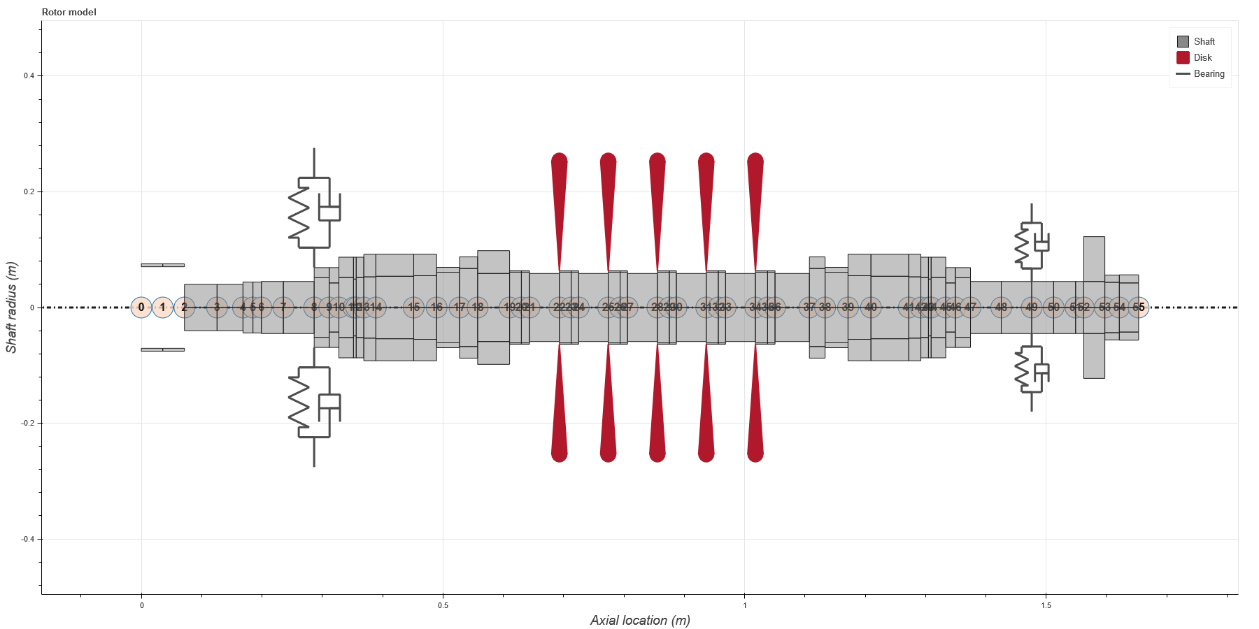
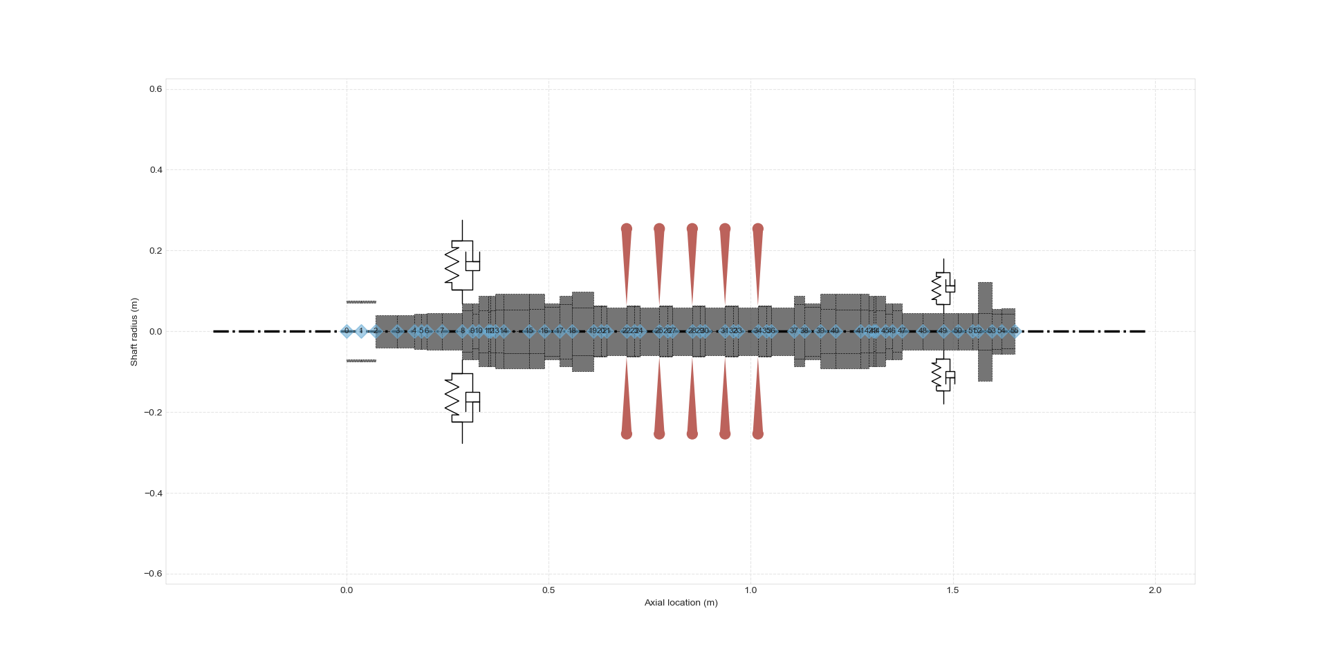
Hover Information for Bearings and Seals#

Added interactive hover information to bearing and seal elements in rotor plots, showing element details on mouse hover — matching the existing shaft element hover functionality.

Bug Fixes#

Fix add_nodes for conical shaft elements#

Fixed incorrect behavior in Rotor.add_nodes when applied to conical (tapered) shaft elements. The method now correctly interpolates diameters and lengths when splitting tapered elements.

Fix transfer matrix for zero-speed FRF#

Corrected the transfer matrix formulation used in frequency response function (FRF) calculations at zero rotation speed, resolving significant discrepancies between numerical and experimental results.

Fix plot_rotor for coupling element#

Fixed an issue that occurred during rotor plotting when a coupling element was combined with bearings.

Fix units in format_table of bearings#

Corrected coefficient units displayed in the .format_table() method of BearingElement subclasses.

Fix TiltingPad class example#

Corrected the example in the TiltingPad class for using the determine_eccentricity equilibrium type, which now requires explicit load inputs.

Fix warning message formatting in TiltingPad#

Fixed formatting of warning messages during TiltingPad initialization.

Fix typos and documentation clarity#

Fixed numerous typos and improved clarity across documentation files, Jupyter notebooks, and Python docstrings.

Documentation and Tutorials#

Added hybrid seal tutorial
Updated AMB sensitivity analysis tutorial (tutorial_part_5) with transfer function methods
Added harmonic balance tutorial with worked examples
Updated multi-rotor and gear element tutorials
Fixed tutorial print output for ShaftElement
Updated README links

Contributors#

This release includes contributions from: @raphaeltimbo, @jguarato, @gsabinoo, @murilloabs, @luisotaviomc2002, @ArthurIasbeck, @Raimundovpn, @ViniciusTxc3, @tches-co

Version 2.0.0#

The following enhancements and bug fixes were implemented for this release:

Enhancements#

Model Reduction#

Added comprehensive model reduction functionality to reduce the size of rotor models while preserving dynamic behavior. Two methods are available:

Guyan reduction: Reduces model to specified degrees of freedom (DOFs)
Pseudo-modal reduction: Uses modal transformation with specified number of modes

The ModelReduction class provides methods to reduce matrices and vectors, and revert reduced vectors back to the full model.

import ross as rs

 compressor = rs.compressor_example()

 dt = 1e-4
 t = np.arange(0, 10, dt)
 speed = 600

 node = [29]
 unb_mag = [0.003]
 unb_phase = [0]

 probe_nodes = [30]

 # Unbalance force
 F = compressor.unbalance_force_over_time(
     node=node, magnitude=unb_mag, phase=unb_phase, omega=speed, t=t
 )

 response = compressor.run_time_response(
     speed,
     F.T,
     t,
     method="newmark",
     model_reduction={
         "method": "guyan",
         "include_nodes": probe_nodes, # Make sure to include output nodes
         "dof_mapping": ["x", "y"],
     },
 )

Thermo-Hydro-Dynamic Tilting-Pad Bearings#

Added two new bearing classes with full THD (Thermo-Hydro-Dynamic) analysis:

TiltingPad: Tilting-pad journal bearing with individual pad analysis, pivot mechanics, and thermal effects. Uses Reynolds equation and energy equation with finite difference methods, Lund’s perturbation method for dynamic coefficients.

ThrustPad: Tilting-pad thrust bearing with similar THD capabilities for axial applications.

Both classes support multiple lubricant types, turbulence modeling, and provide accurate dynamic coefficients for stability analysis.

HolePatternSeal (Annular Seals)#

Added HolePatternSeal class for modeling annular seals with holepattern. Uses bulk flow theory with:

1D compressible flow through annular clearance
Perturbation analysis for dynamic coefficients
Mass, stiffness, and damping matrices
Leakage prediction
Temperature-dependent viscosity using Sutherland’s law

Previously named “honeycomb seal”, this is a comprehensive implementation for pocket damper seals in turbomachinery.

LabyrinthSeal Enhancements#

Significant improvements to the LabyrinthSeal class:

Integration with ccp for gas properties
Support for custom gas mixtures via composition dictionary
Improved numerical methods for pressure distribution
Enhanced velocity field calculations with swirl effects
Up to 10x performance improvement through code optimization

MultiRotor Class#

Added MultiRotor class for analyzing systems with multiple interconnected rotors, such as geared systems. Supports:

Multiple rotors connected via coupling or gear elements
Coordinated modal analysis across all rotors
Campbell diagram for multi-rotor systems
Frequency response analysis
Proper handling of coupled dynamics

GearElement and Mesh Stiffness#

New methodology for gear mesh coupling:

GearElement class for connecting rotors via gear mesh
Mesh stiffness calculation based on gear geometry
Contact ratio computation
Support for multi-rotor analysis with gears

Flexible Crack Models#

Added flexible crack model implementation (breathing and open crack models) for shaft crack analysis. Enables:

Time-varying stiffness due to crack opening/closing
Breathing crack behavior
Open crack model for continuous stiffness reduction

Gravitational Force#

Added gravitational_force() method to apply gravitational loads on the rotor system, useful for static deflection analysis and considering gravity in dynamic simulations.

Free-Free Analysis#

Added free-free boundary condition option in run_freq_response() for analyzing rotors without supports, useful for:

Component mode synthesis
Free-free modal analysis
Validation against experimental modal testing

Torsional Model Conversion#

Added convert_6dof_to_torsional() function to convert a 6-DoF rotor model to a torsional-only model, enabling:

Simplified torsional analysis
Faster computation for torsional-dominated problems
Separate lateral and torsional analysis

Orbit Animation#

Added animation capability to orbit plots with animation=True parameter. Visualizes:

Dynamic motion of the rotor orbit
Time-evolution of displacements
Easier identification of motion patterns

AMB Sensitivity Analysis#

Added run_amb_sensitivity() method for computing Active Magnetic Bearing (AMB) sensitivities according to ISO 14839-3 standard. This enables:

Open-loop, closed-loop, and sensitivity transfer functions calculation
Compliance with API STANDARD 617 stability assessment requirements
Chirp disturbance signal injection for frequency response analysis
Multiple AMB analysis with configurable sensor positions
Time-domain and frequency-domain visualization

The method returns a SensitivityResults object with attributes for magnitude, phase, and maximum sensitivities, plus plotting methods for both frequency-domain (plot()) and time-domain (plot_run_time_results()) visualization.

rotor_amb = rs.rotor_amb_example()

sensitivity_results = rotor_amb.run_amb_sensitivity(
    speed=0,
    t_max=5,
    dt=1e-4,
    disturbance_amplitude=10e-6,
    disturbance_min_frequency=0.01,
    disturbance_max_frequency=150,
    amb_tags=["Magnetic Bearing 0", "Magnetic Bearing 1"],
)

# Access maximum sensitivity for a specific bearing
max_sens = sensitivity_results.max_abs_sensitivities["Magnetic Bearing 0"]["x"]

# Plot frequency response
fig = sensitivity_results.plot()

ROSS GPT Integration#

Integrated ROSS GPT assistant into documentation for interactive help and guidance on using the library.

Performance Improvements#

Significant performance optimizations across multiple modules:

HolePatternSeal Optimization#

Optimized HolePatternSeal for 1.6x faster computation through:

Caching of repeated calculations
Vectorized operations
Reduced function call overhead

LabyrinthSeal Optimization#

Optimized LabyrinthSeal for up to 10x faster performance:

Smart multiprocessing thresholds
Matrix creation optimization
Reduced memory allocations
Efficient array operations

THD Bearing Optimization#

Optimized PlainJournal (THD Cylindrical) bearing calculations using:

Numba JIT compilation for performance-critical sections
Reduced redundant computations
Improved numerical integration

General Optimizations#

Applied lru_cache to frequently-called methods across rotor assembly
Optimized matrix building operations
Reduced computation time in modal and response analyses
Pre-computed base matrices in Rotor.__init__ for faster repeated calculations

API Changes#

Remove 4-DoF Model (Breaking Change)#

Removed support for the 4-DoF model. All analyses now use the 6-DoF model only (lateral, axial, and torsional). This change:

Simplifies the codebase
Ensures consistent behavior across all elements
Improves maintainability
Affects: ShaftElement, DiskElement, BearingElement, PointMass

Migration: Update any code that explicitly used n_dof=4 to work with the 6-DoF model.

Folder Restructuring#

Renamed the fluid_flow folder to bearing for better organization and clarity. All bearing-related classes are now in the ross.bearing module.

Migration: Update imports from ross.fluid_flow to ross.bearing.

Build System Update#

Migrated from setup.py to pyproject.toml for modern Python packaging standards. This improves:

Dependency management
Build reproducibility
PEP 517 compliance

CylindricalBearing Updates#

Enhanced CylindricalBearing class with:

Improved parameter handling
Better documentation with “when to use” guidance
Support for frequency-dependent coefficients
Oil flow properties calculation

Format Table Methods#

Added format_table() methods to results classes for displaying:

Modal analysis results in formatted tables
Bearing coefficients comparison
Critical speeds with detailed information

Check Units Decorator#

Added @check_units decorator to run_* methods for automatic unit validation and conversion, improving:

Type safety with pint quantities
Clear error messages for unit mismatches
Consistent unit handling across methods

Pressure Distribution Plot#

Added pressure distribution plotting capability for THD bearings to visualize:

2D pressure field across bearing surface
Pressure contours
Location of maximum pressure

Documentation and Tutorials#

Documentation Build Updates#

Updated documentation dependencies to latest versions:

Sphinx 7.2.6 → 8.2.3
myst-nb 1.1.0 → 1.3.0
Updated ReadTheDocs Python version to 3.13

Enhanced API documentation with comprehensive theoretical foundations for bearing and seal classes, explaining the numerical methods used.

Tutorial Enhancements#

Expanded tutorials with new examples:

Friswell book examples added to tutorial
MultiRotor usage examples
CouplingElement demonstration
Torsional analysis guide
GearElement examples
New user guide examples (User Guide 30)

Bug Fixes#

Fix integrate_system for Variable Speed#

Fixed NameError in integrate_system() when using variable speed with frequency-dependent bearing coefficients. The bug caused failures in time response analysis with bearings that have speed-dependent properties.

Fix Lund Perturbation Method#

Corrected formulation in Lund’s perturbation method for calculating dynamic coefficients in cylindrical bearings, ensuring accurate cross-coupled stiffness and damping terms.

Fix UCS with Rotor Supports#

Fixed bugs in run_ucs() (Unbalance Constant Speed) analysis when rotor has support elements, including:

Correct equivalent stiffness calculation
Proper DOF handling with supports
Pseudo-modal reduction compatibility

Fix MultiRotor Plots#

Fixed plotting issues for MultiRotor systems, including:

Bearing element visualization
Proper scaling and positioning
Shape updates and reordering

Fix Campbell for Torsional Modes#

Corrected Campbell diagram to properly classify and display torsional modes, preventing misidentification of mode types.

Fix Critical Speed Tracking#

Improved critical speed identification in Campbell diagrams using MAC (Modal Assurance Criterion) to properly track modes across speed range.

Fix Coupling Element Save/Load#

Fixed save() and load() methods for CouplingElement to correctly persist and restore coupling properties.

Fix Misalignment Parameter#

Corrected the sign of the fib variable relationship in flexible coupling misalignment calculations.

Fix Crack Test Precision#

Fixed numerical precision issues in crack test assertions to handle floating-point comparison properly.

Fix plot_deflected_shape Units#

Fixed unit handling in plot_deflected_shape() to properly accept speed as pint Quantity.

Fix Plotly Rendering#

Fixed plotly rendering issues and dropped deprecated heatmapgl traces for compatibility with plotly v6.0.0.

Fix Mode Shape Updates#

Fixed update_mode_3d issue and adapted mode shape plotting methods to work correctly with MultiRotor systems.

Testing and Compatibility#

Python 3.12 and 3.13 Support#

Updated test suite and codebase for compatibility with Python 3.12 and 3.13:

Removed Python 3.9 testing (minimum version now 3.10)
Added Python 3.12 to CI pipeline
Fixed deprecation warnings
Updated dependencies for new Python versions

Contributors#

This release includes contributions from: @raphaeltimbo, @jguarato, @gsabinoo, @ViniciusTxc3, @murilloabs, @Raimundovpn, @gNicchetti, @Emanuela-Carneiro, @vitorp0604, @stanley-washington, @CisneirosRaphael

Version 1.6.0#

The following enhancements and bug fixes were implemented for this release:

Enhancements#

Fix plot torsional and axial modes#

Corrections related to the plotting of mode shapes and includes new methods to handle the plotting of torsional and axial modes in the 6-DoF model.

The plot_with_mode_shape method was not functioning due to changes in the frequency_units parameter in the ModalResults class from previous PRs. To resolve this, corrections were made to manage speed_units separately from frequency_units.

Additionally, new methods were added to the Shape class, including _plot_torsional and _plot_axial, which are now integrated into the plot_mode_2d and plot_mode_3d methods of ModalResults. For 3D plots, an optional animation feature was added, which can be activated by passing animation=True as an argument.

Added CouplingElement#

Added a CouplingElement class that creates a coupling element from input data of inertia and mass from the left station and right station, and also translational and rotational stiffness and damping values. The matrices will be defined considering the same local coordinate vector of the ShaftElement.

API changes#

Change the X Axis (Rotor Speed) in Campbell Diagram#

Now, it’s possible change the x axis (rotor speed) with variable speed_units in plot().

import ross as rs
import numpy as np

Q_ = rs.Q_
rotor = rs.rotor_example()
speed = np.linspace(0, 400, 101)
camp = rotor.run_campbell(speed)
fig = camp.plot(
        harmonics=[1, 2],
        damping_parameter="damping_ratio",
        frequency_range=Q_((2000, 10000), "RPM"),
        damping_range=(-0.1, 100),
        frequency_units="Hz",
        speed_units="RPM",
        )

This PR resolves issue #1087.

Bug fixes#

Version 1.5.0#

The following enhancements and bug fixes were implemented for this release:

Enhancements#

Dev sync ucs map#

For the UCS, the eigenvalues for the synchronous case are now computed directly, eliminating the need to iterate the rotor speed.

Improve numerical integrator#

Newmark method has been added as an option for the numerical integrator used in the .run_time_response() method. Also, the following modifications have been made:

Moved the integrate_system() function from utils.py to be a method of the rotor in rotor_assembly.py.
Added a new ignore argument for constructing the rotor’s $C$ and $K$ matrices. This argument is a list of elements to be disregarded when constructing these matrices.
Provided additional information to the add_to_RHS() function. It is now possible to access, at each time step, the step (required), and optionally, time_step, disp_resp, velc_resp, and accl_resp. For example:

# If you only need to access the step number:
def other_forces(step, **current_state):
    ...

# If you need to access the time step value:
def other_forces(step, time_step=None, **curr_state):
    ...

# If you need to access some response at the current step:
def other_forces(step, velc_resp=None, disp_resp=None, **extra_info):
    ...

# Run time integration:
response = rotor.run_time_response(speed, F, t, method="newmark", add_to_RHS=other_forces)

Enabled the possibility to pass any matrices ($M, C, K, G, K_{sdt}$) as arguments to the function, allowing them to replace the rotor matrices constructed in the code. For example:

# Create new matrices (be careful with the size of the arrays):
M = np.array([...])
C = np.array([...])
K = np.array([...])
G = np.array([...])
Ksdt = np.array([...])

# Run time integration:
response = rotor.run_time_response(speed, F, t, method="newmark", M=M, C=C, K=K, G=G, Ksdt=Ksdt)

Created unit tests (_test_transientnewmark.py) to cover the run_time_response(method="newmark").

Improve Campbell diagram for 6 dof model#

Improved Shape class by adding a new function to classify mode shapes into “Lateral,” “Axial,” or “Torsional.” With the new attribute mode_type, it is now possible to identify the mode shape in the Campbell diagram for the 6 dof model, leading to the creation of two new labels: “Axial” and “Torsional.”

Additionally, an issue was observed in the eigen solver results for certain 6 dof model cases. The sigma argument in las.eigs() function was previously set to 0, which resulted in poor accuracy. By adjusting sigma to a value slightly greater than 0, the accuracy of the results has improved. However, it is not yet clear whether the value now assumed for sigma presents good results for other cases. For more details about this parameter, refer to the solver documentation here.

The values in the hover info of critical speeds were fixed, and I suggested changing the x-axis of the Campbell diagram to “Rotor Speed”.

Some comparison of results are shown below:

Rotor model from tutorial#

LMEst 2 disk rotor#

Gp68#

API changes#

Change defects to faults#

We have renamed the ‘defects’ module to ‘faults’.

Bug fixes#

Fix copying a bearing and setting node#

Fixed a bug when the user tried to copy a bearing and then set it to a different node.

A common requirement is to run an expensive bearing calculation and then copy this bearing and just set a different node where it will be located in the rotor:

import ross as rs
from copy import copy

bearing_de = rs.SpecialBearing(n=0, ...)
bearing_nde = copy(bearing_de)
bearing_nde.n = 20

The above code would give an error, since in the rotor assembly we have code which relies on bearings having n_l and n_d attributes (although this only makes sense for shaft elements).

This code removes the attribute from bearing initialization and sets it at rotor initialization. This way it is possible to modify the attribute before creating the rotor.

Fix y label for frequency response plots#

Fixed the y label for the frequency response plots, showing ‘magnitude’ instead of displacement, velocity or acceleration.

Fix use of Kst matrix#

Corrected the stiffness matrix Kst resulting from the transient motion. This matrix should be multiplied by the acceleration, rather than the rotor speed as was previously done.

Fix disk K matrix#

The K matrix for the disk elements should be zero. In the 6 dof model, there was confusion between the K matrix and the Kdt matrix of disk elements. This PR resolves this misunderstanding. Additionally, it proposes the incorporation of the Kdt matrix into the rotor Ksdt matrix, which represents the stiffness matrix related to transient motion of the shaft and discs (formerly Kst).

Fix 6 dof matrices#

the signs of K and M matrices of the shaft elements;
the consideration of shear effect on M matrix of the shaft elements;

Fix run_ucs for 6 dof model#

Closes issues #1034 and #772

Fixed the run_ucs() method to not show the axial and torsional modes in the 6 dof model results. A new function has been added to utils.py to convert a 6 dof rotor model to a 4 dof model to support this update.

Comparisons of old UCS maps are presented below with those obtained after modification:

rotor.run_ucs(stiffness_range=(6, 11), num=20, num_modes=16)

rotor.run_ucs(stiffness_range=(6, 11), num=20, num_modes=24)

Version 1.4.0#

The following enhancements and bug fixes were implemented for this release:

Fix the y label for the frequency response plots, showing ‘magnitude’ instead of displacement, velocity or acceleration.

Documentation improvements in the tutorials and class/functions missing from the API reference.

Version 1.3.0#

The following enhancements and bug fixes were implemented for this release:

Enhancements#

Python 3.10 support#

This release adds Python 3.10 support.

Version 1.2.0#

The following enhancements and bug fixes were implemented for this release:

Enhancements#

Added Shape and Orbit classes#

We have added a Shape and an Orbit class to the results module. These classes are now responsible for calculating the mode shapes in the ModalResults class and also the deflected shapes in the ForcedResponseResults class. This simplifies the code since it avoids the repetition of code between these two classes. It also selects a single method for calculation of the major/minor axes and precession (forward or backward). Before, in the ModalResults, we were doing this using the method described by Friswell with the eigenvalues of the H matrix, and in the ForcedResponseResults we were using a calculation based on forward and backward vectors. The current code in the Orbit uses the method described by Friswell.

Bug fixes#

Fix ucs map#

Fix calculation of bearing stiffness for plotting

Since we have removed the Coefficient class we no longer calculate the bearing coefficient with bearing.kxx.interpolated. Now we use bearing.kxx_interpolated.

Fix number of modes

It was only possible to plot 4 modes. Now we can change the num_modes which is the number of calculated modes, and we will have that value divided by 4 being plotted. Value is divided by 4 because for each pair of eigenvalues calculated we have one wn, and we show only the forward mode in the plots, therefore we have num_modes / 2 / 2.

Fix stiffness expression for tapered element#

In the stiffness expression described on appendix A of the Genta and Gugliotta paper, when substituting chi = 12EI/(phiGA*L**2) in the constant that multiplies the second matrix, we had canceled the A here with the Aj from the equation, but they are actually not the same area. The area Aj in the equation refers to the area in the element’s left side, while the area in the chi calculation refers to the area in the middle of the element. Therefore, we were having an error in this formula by a factor of Aj / A.

Version 1.1.0#

The following enhancements and bug fixes were implemented for this release:

Enhancements#

Removed python 3.6 support#

Since we are now using pint 0.18 which requires python 3.7+, we can no longer support python 3.6.

Add damping parameter and filtering to campbell#

Three additional arguments have been added to the Campbell plot:

damping_parameter: choose between log_dec or damping_ratio;
frequency_range: filter out modes that are out of this frequency range;
damping_range: filter out modes that are out of this damping range;

Improve bearing save method#

Save and load methods for bearings have been modified in order to have additional info in the save file, such as attributes used in bearing initialization.

API changes#

Change pkpk parameter used in plot#

The peak to peak parameter (pkpk) has been changed from prefix to constant, which simplifies it use. To use peak to peak use ‘<unit> pkpk’ (e.g. ‘m pkpk’)

Remove coefficient class#

Remove the auxiliary _Coefficient class in favor of a more simple data processing within the BearingElement class. The _Coefficient class was used to process the coefficient data, creating the interpolation functions and also providing plots (e.g. bearing.kxx.plot()). This was making the code more complicated since we basically had to reproduce the methods of an iterable object in this class. The discoverability of the plot function was also improved, since it is more natural for the user to search for a plot function within the bearing element and not as an attribute of each coefficient (bearing.plot('kxx') instead of bearing.kxx.plot() is now used). Another improvement regarding the plot is that the user can now pass multiple coefficients to plot with. Before the user would have to do something like:

fig = bearing.kxx.plot()
fig = bearing.kyy.plot(fig=fig)
fig = bearing.kxy.plot(fig=fig)
fig = bearing.kyx.plot(fig=fig)

Now we can do:

bearing.plot(coefficients=['kxx', 'kyy', 'kxy', 'kyx'])

Bug fixes#

Correct an error in the damping coefficient of the Magnetic Bearings Element#

A small error in the magnetic bearing calculation has been corrected. See #816.

Fix error in static analysis for bearings with high stiffness#

This adds an auxiliary rotor with 0 stiffness in the bearing location to fix calculations, otherwise, a rotor with a bearing with high stiffness would have 0 reaction force at the bearing location.

Fix error in static analysis for bearings and disks added to the same node#

For rotors with a bearing and a disk added to the same node the static analysis would fail. See #845 for more details.

Version 1.0.0#

The following enhancements and bug fixes were implemented for this release:

Enhancements#

Add loop to calculate frequency-dependent coefficients in from_fluid_flow()#

Users will be able to input as many frequency values as needed and from_fluid_flow() will run a loop calculating a set of coefficients for each given frequency. Now, omega argument must be a list of frequencies. It also changes the main function used to calculate the coefficients. calculate_stiffness_and_damping_coefficients() is now used to do it numerically.

Extract fluid flow#

The .from_fluid_flow method has been extracted from the BearingElement to a class called BearingFluidFlow. This is more in line with how we have all the Bearing classes, and makes it easier for the user to find it.

Add minor and major axes to response plots#

We can now select the major and minor axis when plotting responses:

   # plot response for major or minor axis:
   >>> probe_node = 3
   >>> probe_angle = "major"   # for major axis
   >>> # probe_angle = "minor" # for minor axis
   >>> probe_tag = "my_probe"  # optional
   >>> fig = response.plot(probe=[(probe_node, probe_angle, probe_tag)])

Calculate velocity and acceleration responses

The method run_freq_response() now returns, not only the displacement results, but also the velocity and acceleration. The data is then input to FrequencyResponseResults and ForcedResponseResults classes.

The user is able to choose the response by changing the amplitude_units argument.

Inputing ‘[length]/[force]’, it displays the displacement;
Inputing ‘[speed]/[force]’, it displays the velocity;
Inputing ‘[acceleration]/[force]’, it displays the acceleration.

Add units to stochastic ross module#

Units use is now possible in the stochastic module.

Crack, rubbing and misalignment simulation#

It is now possible to run simulations for some defects such as cracks, rubbing and misalignment.

API changes#

Change methods to run_#

The plot_level1 and plot_ucs methods were refactored so that they behave as other run methods. Now we use the run* prefix to call them and they will return Results objects.

ucs = rotor.run_ucs(...)
ucs.plot(...)

Bug fixes#

Fix GlobalIndex with non integer values#

PointMass and BearingElements with n_link argument were getting non integer values. Matrices would not be built, once these values are used as reference to array indexes (which must be integers).

Fix DoF error when using “n_link”#

Add link_nodes attribute to Rotor object that holds the nodes created using n_link
Correct DoFs with link_nodes in ForcedResponseResults and TimeResponseResults

Version 0.4.0#

The following enhancements and bug fixes were implemented for this release:

Enhancements#

Class MagneticBearingElement was created#

This class creates a magnetic bearing element. The element can be created by:

defining directly the stifness and damping coefficients with the method **init**;
defining the magnetic parameters g0, i0, ag, nw, alpha and the proportional and derivative gains of a PID controller kp_pid, kd_pid with the method param_to_coef.

The reference for the equations is: Book: Magnetic Bearings. Theory, Design, and Application to Rotating Machinery Authors: Gerhard Schweitzer and Eric H. Maslen Page: 84-95 (magnetic parameters) and 354 (PID gains)

Stochastic Ross module#

The files follow the hierarchy of ROSS: different files to build the elements and a main file to build the rotors.

The main difference between these new files and the element files from ROSS is that the stochastic elements files build a list of elements instead of a single one.

The analysis will also follow the ROSS structure, but it’s not added yet.

6dof assembly#

Generalization of the assembly and evaluation codes of ROSS for a generic “N” DoF sized formulation. This is intended to enable the 6 DoF implementation to be executed appropriately, and is made in a generalized fashion by default.

Add scale_factor argument to DiskElement class#

Argument to scale the disk patch. Used to increase (scale_factor > 1.0) or reduce (scale_factor < 1.0) the size of disk patches when plotting the rotor.

Add units to the DiskElement, BearingElement and PointMass classes#

Arguments for these classes can be passed as pint.Quantity now.

Replacing plotting libraries#

We have replaced Matplotlib and Bokeh plotting libraries with Plotly.

Add methods to plot the deflected shape

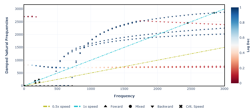
Set default values to log_dec color scale#

The color scale to represent the log_dec values ranges between 0 and 1, independently of the log_dec values calculated. It can be manually modified by insert 2 simple kwargs: coloraxis_cmin and coloraxis_cmax. It will change respectively the minimum and maximum values for the color scale. Also adds exponentformat = “none” to X and Y axis for better visualization of values

Example with default options:

>>> speed_range = np.linspace(0, 3000, 51)
>>> campbell = rotor.run_campbell(speed_range)
>>> campbell.plot(harmonics=[0.5, 1])

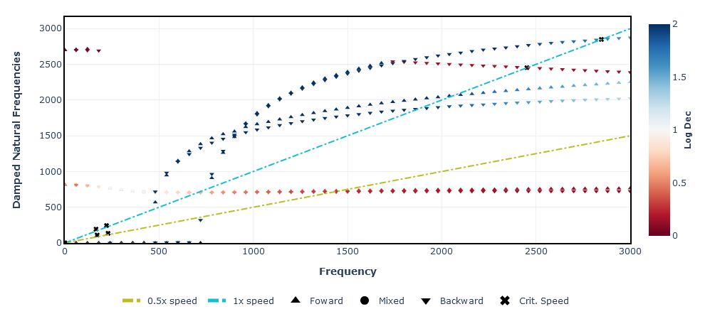
Example changing the max value for the scale:

>>> speed_range = np.linspace(0, 3000, 51)
>>> campbell = rotor.run_campbell(speed_range)
>>> campbell.plot(harmonics=[0.5, 1], coloraxis_cmax=2.0)

Replace interp1d by line_shape from Plotly#

It removes the need of creating sub arrays from interpolation to smooth some results in StaticResults.

Add probe argument to ForcedResponseResults#

Replace dof by probeargument probe is a list of tuples. Each tuple refers to a probe, which must include the node and the orientation.

The orientation units is set by probe_units argument. in plot() method, data.showlegend is turn off to avoid repetitive legend marks on graphs

Change .use_material() to .load_material()#

We have change most methods to use the word ‘save’ and ‘load’ instead of ‘get’, ‘use’ etc.

Move “sparse” argument to run_modal()#

The eigenvalue / eigenvector solver is chosen when running the run_modal() method, and is no longer a parameter from the rotor model

Bug fixes#

Fix issue with check_units#

Related to Issue #511

Add a condition to verify if the argument value is None. It allows the user to pass “None” args without getting an error with the code trying to assign a unit to a None value.

Fix missing parameters in ST_ShaftElement#

The parameters axial_force and torque were missing from the ST_ShaftElement.__init__().

Fix missing y_pos and y_pos_sup in df_seals#

Related to Issue #571.

Seals can be displayed in different colors than bearings

Fix ValueError when inputting an integer to disk properties#

Related to Issue #593.

Version 0.3.0#

The following enhancements and bug fixes were implemented for this release:

Enhancements#

Remove ShaftElement and replace with the ShaftTaperedElement#

Now we only have one class for the shaft element which is capable of handling cylindrical and tapered elements.

Allow user choose material in “Rotor.from_section()”#

As requested in Issue #401, the user will be able to define a material when using .from_section() classmethod. In addition, more modifications have been done regarding the new ShaftElement API. Now, the user has the option to instantiate tapered sections.

CoAxialRotor class#

A class is now available for modeling coaxial rotors.

Bug fixes#

Fix links not working for more than one support#

Related to Issue #382.

We were having problems defining the global indexes for the elements using this method internally in an element class. It makes more sense to use .dof_global_index() when build the rotor model. The routine to calculate the elements’ global indexes have been moved to rotor_assembly (.__init__() method). Now, each element has an attribute that keeps those index, instead of calling a function to this job.

Fix bearing position bug#

Fix bug mentioned in Issue #276

Sorting the bearing_seal_elements make it to cycle correctly while assuming y_pos values to them.

Version 0.2.0 (beta release)#

The following enhancements and bug fixes were implemented for this release:

Enhancements#

Improvements for plotting results#

This PR make some modifications in results.py

Add show(camp) to show campbell bokeh plotting
Add command to align ColorBar axis for better appearance
Add figure dimensions for campbell bokeh plotting
increases the font size of all axis labels

Some bokeh figures have the attribute sizing_mode="stretch_both. This command line is used so that the plotting of the graphics is always the maximum size of the browser. However, this creates a bug in jupyter notebook, and the graphs does not appears. So it should be replaced by width and height command lines

adds an interpolation function to highlight to the user the intersection between the critical frequency curves and the speed line

Index method#

Adds .dof_local_index() and .dof_global_index() methods to the elements. These methods will return namedtuples with the index for each coordinate based on the following convention:

As an example:

>>> import ross as rs
>>> from ross.materials import steel

>>> le = 0.25
>>> i_d = 0
>>> o_d = 0.05
>>> sh_el = rs.ShaftElement(le, i_d, o_d, steel, n=2)
>>> sh_el.dof_local_coordinates()
LocalIndex(x0=0, y0=1, alpha0=2, beta0=3, x1=4, y1=5, alpha1=6, beta1=7)
>>> sh_el.dof_global_coordinates()
GlobalIndex(x0=8, y0=9, alpha0=10, beta0=11, x1=12, y1=13, alpha1=14, beta1=15)

With this we can change the following code:

for elm in self.shaft_elements:
    n1, n2 = self._dofs(elm)
    M0[n1:n2, n1:n2] += elm.M()
for elm in self.disk_elements:
    n1, n2 = self._dofs(elm)
    M0[n1:n2, n1:n2] += elm.M()

To:

for elm in self.elements:
    dofs = elm.dof_global_index()
    n0 = dofs[0]
    n1 = dofs[-1] + 1  # +1 to include this dof in the slice
    M0[n0:n1, n0:n1] += elm.M()

interactions with rotor plotting#

When plotting a rotor, the user will be able to check some parameters of the elements in the output image itself, just by moving the cursor over the desired element, for example:

By moving the cursor over a shaft element the user will see this:

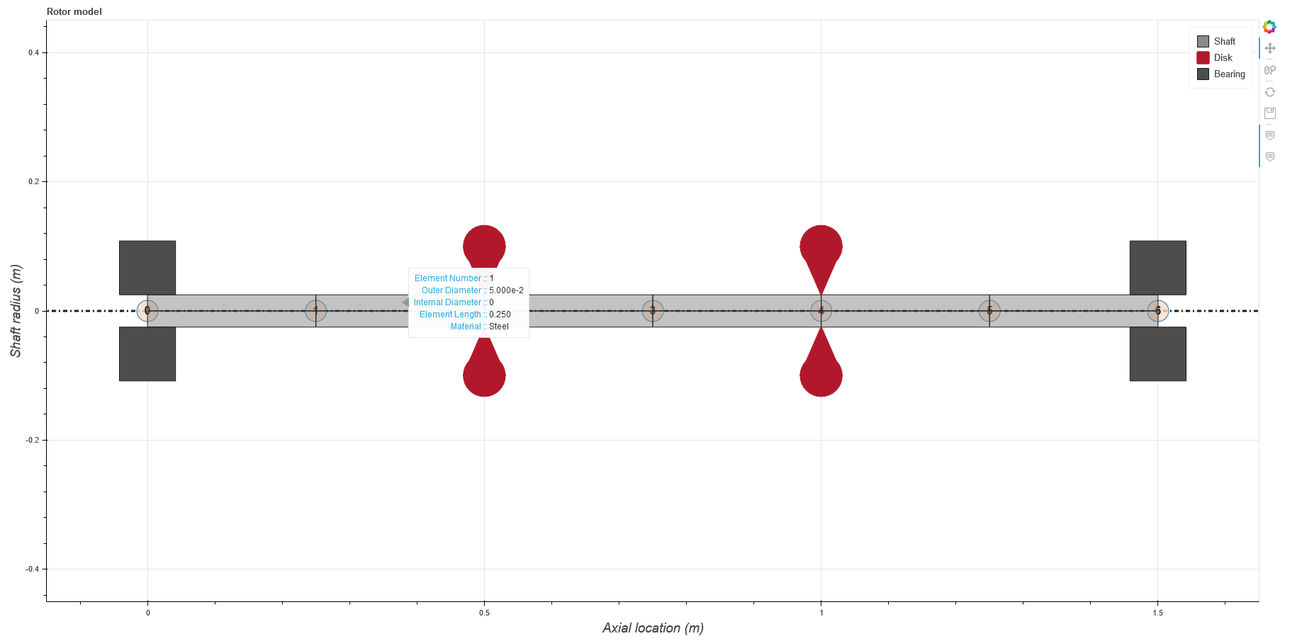
And, by moving the cursor over a disk element the user will see this:

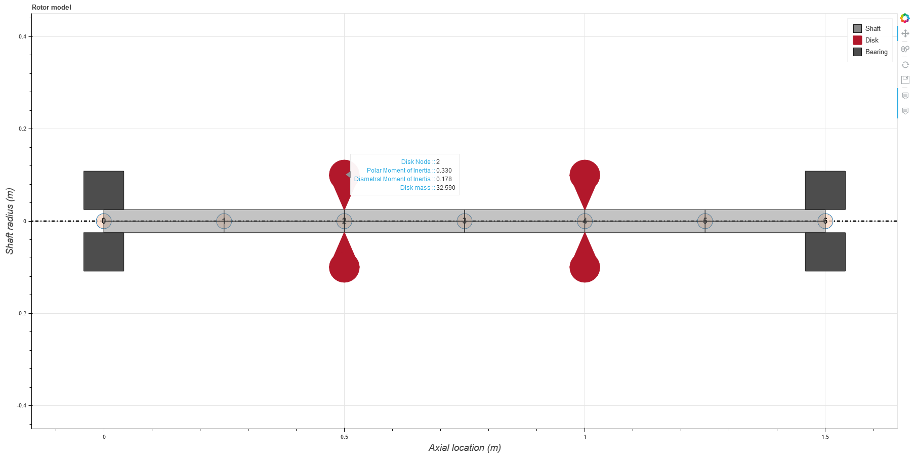
I didn’t add the same functionality to bearing elements because the coefficients may vary with rotor speed, and this may cause a misunderstanding to the user.

Move time response plotting to results#

Removes the code related to plotting from this file. It was transfered to results.py
Replaces the method name from plot_time_response to run_time_response.
Fix ForcedResponseResults docstring

Add tapered shaft element#

Add new element: tapered shaft element
Add class ShaftTaperedElement
This class have, basically, the same inputs than “ShaftElement”. The difference relies on entering the diameters of each side of the element (left and right).
Patches methods were adapted to draw the conical shape of the element.

The matrices generated for this element follow the reference below.

Genta, G., and Gugliotta, A. (1988). A conical element for finite element rotor dynamics, Journal of Sound and Vibration 120,175-182.

Improving plot rotor#

This PR modifies the plotting size of disks, bearings and seals. The size, previously based on shaft length, is now calculated based on the shaft diameter.

Add Check slenderness ratio method#

Adds a method that will return the colored rotor plot if the condition to the mininum slenderness ratio is not met.

Now using .plot.rotor() won’t display the colored rotor anymore. Instead, the user will call .check_slenderness_ratio() to check this attribute.

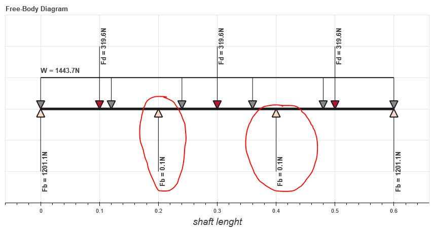
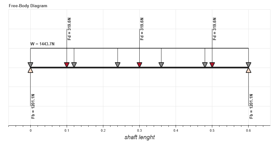
Make Free-Body Diagram more readable#

Pull Request to fix Issue #243

Slightly increases the size of the figures
Arrows have a fixed length now (as shown in this figure below);
Arrows now have different colors to distinguish forces (from shaft, disks or bearings/seals);
Labels were rotated 90º;
Text font size reduced to “9pt”;
Y axis is hidden. The force values are only displayed only next to the arrows, without size ratio.

Replace bearing plot style / remove element length dependency from glyphs#

Bearing representation changes from a simple square to a spring-damper set.
Fix bug glyphs were plotted on the minimum outer diameters of a shaft node.
Removes length attribute from patch() and bokeh_patch() of BearingElement and DiskElement classes.

Bokeh plot

Matplotlib plot

Add API_report#

Work in Progress

This PR adds some plotting styles following the API reference:

Separation Margin
Amplification Factor
Table of API parameters

It follows the Issue #195

Add new “Tag” attribute to elements#

Disk, bearing and seal elements now get an attribute called “Tag”. This allows the user to name the elements to help refer to the actual equipment (impellers, blades, labyrinth seal…)

If the user do not input a tag, it’s named after:

Disk 1, 2, 3…
Bearing 1, 2, 3…
Seal 1, 2, 3…

As bearings and seals are input in the same list of objects, this situation below may happens:

def rotor_example():
    i_d = 0
    o_d = 0.05
    n = 6
    L = [0.25 for _ in range(n)]

    shaft_elem = [
        ShaftElement(
            l, i_d, o_d, steel, shear_effects=True, rotary_inertia=True, gyroscopic=True
        )
        for l in L
    ]

    disk0 = DiskElement.from_geometry(
        n=1, material=steel, width=0.07, i_d=0.05, o_d=0.28
    )
    disk1 = DiskElement.from_geometry(
        n=3, material=steel, width=0.07, i_d=0.05, o_d=0.28, tag="disk_test"
    )
    disk2 = DiskElement.from_geometry(
        n=5, material=steel, width=0.07, i_d=0.05, o_d=0.28, tag="disk_test2"
    )

    stfx = 1e8
    stfy = 1e8
    bearing0 = BearingElement(0, kxx=stfx, kyy=stfy, cxx=1000, tag="brg")
    bearing1 = BearingElement(6, kxx=stfx, kyy=stfy, cxx=1000)
    seal0 = SealElement(2, kxx=1e2, kyy=1e2, cxx=500, cyy=500, tag="seal")
    seal1 = SealElement(4, kxx=1e2, kyy=1e2, cxx=500, cyy=500)

    return Rotor(shaft_elem, [disk0, disk1, disk2], [bearing0, seal0, seal1, bearing1])

>>> rotor = rotor_example()
>>> rotor.df_bearings["tag"]
0    brg
1    seal
2    Seal 2
3    Bearing 3
Name: tag, dtype: object

The counting for bearings and seals is not independent. I don’t see it as big deal, but I’m open to suggestions.

Add separated DataFrame to seals#

This splits bearings from seals in two different dataframes:

df_bearings for bearings
df_seals for seals

It aims to better organize the elements and to avoid code interpretation problems such as in static analysis:

This is the free-body diagram of an example while seals and bearings are merged in same dataframe. The code interprets seals like bearings and calculate reaction forces where both seals are placed:

And now, spliting bearings and seals:

Also, fix a bug when modeling too flexible bearings, displacement were getting larger than acceptable. It uses auxiliary bearings with high stiffness, considering almost zero displacement in bearing nodes.

Split StaticResults plot method#

This commit splits the plot method in four:

plot_deformation()
plot free_body_diagram()
plot_shearing_force()
plot_bending_moment() This is related to Issue #303.

Add BallBearing and RollerBearing Element#

This PR adds two new classes:

BallBearingElement
RollerBearingElement

These classes create a bearing element for ball and roller bearings models. They are instantiated based os some geometric and constructive parameters like: number of rotating elements, size (diameter for ballbearing; length for rollerbearing) of the rotating elements, contact angle, and static loading force.

The direct stiffness coefficients are calculated using these parameters.

I also left an opened option to instantiate the direct damping coefficients. But if it’s set as None, they are calculated based on the stiffness coefficient as the literature suggests. However the cross-coupling coefficients are set to zero, and the coefficients are not dependent on speed.

def __init__(
    self,
    n,
    n_balls,
    d_balls,
    fs,
    alpha,
    cxx=None,
    cyy=None,
    tag=None,
):

    Kb = 13.0e6
    kyy = (
        Kb * n_balls ** (2./3) * d_balls ** (1./3) *
        fs ** (1./3) * (np.cos(alpha)) ** (5./3)
    )

    nb = [8, 12, 16]
    ratio = [0.46, 0.64, 0.73]
    dict_ratio = dict(zip(nb, ratio))

    if n_balls in dict_ratio.keys():
        kxx = dict_ratio[n_balls] * kyy
    else:
        f = interpolate.interp1d(nb, ratio, kind="quadratic")
        kxx = f(n_balls)

    if cxx is None:
        cxx = 1.25e-5 * kxx
    if cyy is None:
        cyy = 1.25e-5 * kyy

    super().__init__(
        n=n,
        w=None,
        kxx=kxx,
        kxy=0.0,
        kyx=0.0,
        kyy=kyy,
        cxx=cxx,
        cxy=0.0,
        cyx=0.0,
        cyy=cyy,
        tag=tag,
    )

Add condition to ShaftTaperedElement instantiation#

Add a condition if the user do not attribute any value to inner and outer diameters on the right side, the values are automatically set to be equal the left side.
Also, move the “material” input to the first position, so the geometric parameters can be grouped together.
Adapt the examples in docstring.

Moves the inputs from ShaftTaperedElement to match the new position set.

class ShaftTaperedElement(Element):
  def __init__(
      self,
      material,
      L,
      i_d_l,
      o_d_l,
      i_d_r=None,
      o_d_r=None,
      n=None,
      axial_force=0,
      torque=0,
      shear_effects=True,
      rotary_inertia=True,
      gyroscopic=True,
      shear_method_calc="cowper",
      tag=None,
  ):

      if i_d_r is None:
          i_d_r = i_d_l
      if o_d_r is None:
          o_d_r = o_d_l

Patches for PointMass element#

As required by issue #310

Add repr, eq, and example() to point mass element#

This commit adds the following methods to PointMass class:

repr - representative method;
eq - comparison method;
point_mass_example() - to run some doctests.

Improvements to Static Analysis Documentation#

Related to Issue #327
Remove force_data dictionary
Get the items and transform them in Rotor attributes
- shaft_weight - Shaft total weight
- disk_forces - Weight forces of each disk
- bearing_reaction_forces - The static reaction forces on each bearing

General Modifications in CampbellResults#

This is related to Issues #326 and #328.

Introduce a condition to add the hover tool only if an harmonic crosses a critical speed curve.
Remove some unused imports.
In _plot_bokeh:
- Change colormap from viridis to Red-Blue
- Add different colors to harmonics lines
- Make glyphs on legend with same color
In _plot_matplotlib:
- Add different colors to harmonics lines
For both methods: Restructure code to increase efficiency (reduce plotting time): I could the plot time in an half by rearranging some routines.

import ross as rs
rotor = rs.rotor_example()
camp = rotor.run_campbell(np.linspace(0, 1000, 10)).plot([0.25, 0.5, 1, 2])
show(camp)

I’ve measured the time just to run the .plot(). It was taking 2.5s for the rotor_example(). Rearranging the code, it has been reduced to 1.2s for this same example.

Add summary table to plot rotor information#

Related to Issue #327.

It’s a first idea from what the summary will become. The class get the values stored in dataframes and turns them into a bokeh widget in table format.

We still can build other tables to make it more complete and useful to manipulate data.

Improvements to SummaryResults#

Related to Issue #327 Follows the PR #338

Add new attribute “tag” to name the rotor;
Add CG and Moment of Inertia parameters;
Add new attributes to .summary() method;
Add a system of Tabs that allows the user to alternate between tables;
Tables are separeted in:
- Rotor summary
- Shaft summary
- Disk summary

Add Stability Level 1 analysis#

This analysis consider a anticipated cross coupling QA based on conditions at the normal operating point and the cross-coupling required to produce a zero log decrement, Q0.
Add attribute “rotor_type”
- This attribute is necessary to distinguish overhung and between bearings rotors.
- The unbalance forces and the respective nodes where they are introduced depend on this information.
Improve unbalance force method.
- With this improvement, the unbalance forces are calculated according to the rotor_type and considers the disks and shaft weight (if overhung).
Change mode_shape to find nodes according to rotor_type
- The method .mode_shapes() was capturing the maximum points from the rotor’s mode shapes without checking if it was overhung or between bearings.
- For rotors where the disk is cantilevered beyond the bearings, unbalance shall be added at the disk. So, the method now checks the rotor_type to define the nodes correctly.
Add machine_type and disk_nodes attribute
- Machine_type will be useful to help the code to distinguish between compressors, turbines, etc. Because each machine type has their own conditions to be calculated.
- Disk_nodes is useful to collect the disk of interest. if we are working with a overhung rotor, disk_nodes will collect the disk which are overhung only, for example.

This Level 1 analysis does not have the screening criteria yet. The next step is to implement the Level 2 analysis. Once I get to work on it, I’ll add the screening criteria. I still need to organize some ideas for the next step.

Add Bearing Summary Table#

add a summary table for bearing elements: for now it displays only where it’s placed and the reaction forces.
fix bug: when setting and disk or bearing element in the last node, the code would fail
other minor changes

Improvements to api_report.py - Add test_api_report.py#

Add Stability level 1 screening criteria;
Modifies the code to storage the cross-coupling range for each rotor stage (or impeller). This is useful to distinguish the cross-coupling evaluation for different rotor_types (between bearings, overhung…);
Add .summary() method;
Add summary for stability level 1

Add stability analysis level 2#

For the level 2 stability analysis additional sources that contribute to the rotor stability shall be considered. These sources shall replace the cross-coupling Qa, calculated in the stability analysis level 1

Visual improvements to graphs#

The labels, ticks and titles font size from bokeh figure were small when putting it presentations. So I’ve increased the font size of all graphs.

Add new tab to the .summary() with stability level 2 data;
Change stability level 2 labels for better user understanding when using .summary(). The labels include explicitly all the components considered in a certain analysis (Shaft + Bearing + Disk + Seal…);
Increases labels, titiles and tick font sizes (results.py and api_report.py);
Add mcs speed to evaluate mode shapes (api_report.py);
Fix .unbalance_response() plot size to match results.py file;
In .stability_level_1() remove condition from returning and add it as attribute;
.run_modal().plot_mode() add legend informing the whirl direction.

Add method to plot orbit#

Add .run_orbit_response() method to rotor_assembly.py.
- .run_orbit_response() calculates the orbit for a rotor’s given node, speed and forces.
Add class OrbitResponseResults to results.py.
- Class used to store results and provide plots for orbit response.

Example using this new method:

>>> rotor = rotor_example()
>>> speed = 500.0                                           # pick a rotor speed
>>> size = 10000                                            # time array's size
>>> node = 3                                                # node of interest
>>> t = np.linspace(0, 10, size)                            # create time array
>>> F = np.zeros((size, rotor.ndof))                        # create force vectors
>>> F[:, 4 * node] = 10 * np.cos(2 * t)                     # introduce a periodic force in a single dof
>>> F[:, 4 * node + 1] = 10 * np.sin(2 * t)                 # introduce a periodic force in a single dof
>>> response = rotor.run_orbit_response(speed, F, t, node)  # run orbit response
>>> show(response.plot())                                   # plot orbit response

3D plots for orbit response#

Related to PR #385.

API changes#

Bug fixes#

Fix Campbell’s strange behavior for precession

Fix equality for bearing element#

Fixes the equality for bearing element, allowing the comparison with objects from different types, e.g. bearing == 1 will return False, before an AttributeError was raised since int doesn’t have .dict. This also removes pytest as a dependence for the user.

Add import to Axes3d#

The import has been added to the results module because the mode shape plot needs this to work. Although it looks like the import is not being used (this is highlighted by linters), matplotlib, for some strange reason, actually needs this to use the projection=’3d’. A doctest has been added to the mode shape plot for the tests to fail if this import is removed.

Fix bearing type definition and add new test#

Fix the bearing type definition and also add a new test that checks if a second analytical way to calculate the pressure matrix matches the numerical way. Close #175

Improvements for plotting results#

This PR make some modifications in results.py

Add show(camp) to show campbell bokeh plotting
Add command to align ColorBar axis for better appearance
Add figure dimensions for campbell bokeh plotting
increases the font size of all axis labels

Some bokeh figures have the attribute sizing_mode="stretch_both. This command line is used so that the plotting of the graphics is always the maximum size of the browser. However, this creates a bug in jupyter notebook, and the graphs does not appears. So it should be replaced by width and height command lines

adds an interpolation function to highlight to the user the intersection between the critical frequency curves and the speed line

Fix bug - plotting unbalance response#

Unbalance response was not plotting when calling it using matplotlib

Make Free-Body Diagram more readable#

Pull Request to fix Issue #243

Slightly increases the size of the figures
Arrows have a fixed length now (as shown in this figure below);
Arrows now have different colors to distinguish forces (from shaft, disks or bearings/seals);
Labels were rotated 90º;
Text font size reduced to “9pt”;
Y axis is hidden. The force values are only displayed only next to the arrows, without size ratio.

Fix inconsistencies in the mass and gyroscopic matrices; New tests for shaft tapered element

I found some problems in shaft tapered element matrices. Fow now I’ve fixed the issues on mass and gyroscopic matrices. Besides this PR modifies the tests for this class, adding tests to compare two cylindrical elements built from ShaftElement and ShaftTaperedElement classes. However, tests for stiffness matrices are skipped.

Fix typo in repr#

It follows the Issue #255.

Fix inconsistencies in the stiffness matrix#

Fix some typos in geometry coefficients;
Fix stiffness matrix formula for shaft tapered elements;
Fix docstrings for M(), K(), G() in ShaftTaperedElement;
Add better docstrings to ShaftTaperedElement.

Fix tests to match the changes done in shaft_element.py:

Fix stiffness matrix test;
Fix element attribute tests ;
Fix comparation tests.

Fixing doctests#

Well, since I have forgotten to add the .py extention on api_report file, the CI’s were not running the tests on it. And now that I did it, the building is failing due some tests.

This PR tries to fix this problem on api_report.py and in results.py (with new docstrings on ModeShapeResults)

The last PR (#272) was a failure actually.

Adapt convergence analysis to ShaftTaperedElement#

Now the convergence analysis uses the class ShaftTaperedElement to generate shaft elements since it’s more generic. This should solve issue #280.

Add separated DataFrame to seals#

This splits bearings from seals in two different dataframes:

df_bearings for bearings
df_seals for seals

It aims to better organize the elements and to avoid code interpretation problems such as in static analysis:

This is the free-body diagram of an example while seals and bearings are merged in same dataframe. The code interprets seals like bearings and calculate reaction forces where both seals are placed:

And now, spliting bearings and seals:

Also, fix a bug when modeling too flexible bearings, displacement were getting larger than acceptable. It uses auxiliary bearings with high stiffness, considering almost zero displacement in bearing nodes.

Fix warning when changing number of nodes to be plotted#

Related to Issue #295

Remove unit conversion factor#

Remove a conversion factor (meters to milimeters) from the plot_deformation() ColumnDataSource. So the x and y axis units get to be the same.

Related to Issue #312

Improvements to Static Analysis Documentation#

Related to Issue #327
Remove force_data dictionary
Get the items and transform them in Rotor attributes
- shaft_weight - Shaft total weight
- disk_forces - Weight forces of each disk
- bearing_reaction_forces - The static reaction forces on each bearing

Fix bearings not connecting to tapered elements#

Related to Issue #332

Fix bug when plotting bearings#

Fix bug when plotting bearing elements in a given node with more than 1 shaft element on it. The bearing would not get correct starting point.
Fix bug when using scale_factor with point mass. The auxiliar bearing would disattach from the first bearing.

Fix bug in .run_freq_response()#

Fix a bug that happens when calling .run_freq_response() with default arguments, i.e:

>>> rotor = rotor_example()
>>> response = rotor.run_freq_response()
Traceback (most recent call last):

  File "<ipython-input-3-292fe59ccc9e>", line 1, in <module>
    response = rotor.run_freq_response()

AttributeError: 'NoneType' object has no attribute 'imag'

Since running .run_modal() is required to create the attribute evalues, we need to call this function (run_modal()) before creating a default speed_range based on the evalues.

This should fix it.

Version 0.1.0 (alpha release)#

For the alpha release, the main classes have been created and the more important analyses have been implemented.

The following gives a list of enhancements, api changes and bug fixes that were implemented for this release:

Enhancements#

Implementation of the Material class#

A class has been implemented to represent any material that can be used when creating an element for the analysis.

Create ShaftElement, DiskElement and BearingSealElement#

The main classes used to create shaft elements, disk elements and bearings/seals elements have been implemented.

Add rotor assembly and results#

A Rotor class has been implemented to represent the rotor. A rotor object assembles the global matrices and provides methods to run the same analysis on the rotor. Results implemented are modal analysis, Campbell, frequency response and unbalance response.

Add static analysis method#

A method to calculate the static displacement of a rotor due to disks’ weight has been added.

New rotor save format#

A new format for saving rotors was implemented. It is based on the toml format.

Add convergence analysis#

Add convergence analysis as a method to the class Rotor.

Analytical fluid flow, short bearings#

Add analytical fluid flow routines for short bearings.

Add new diagram to static method#

Add a new plot to the static method - shearing force and changes the name of some graphs to make it more readable.

Add methods to allow inputs from a table in bearing element#

Two methods were added to bearing element. The first one allows instantiating a bearing object from a table (excel format). The second one converts from table to dictionary, that can be saved as a toml file.

Interpolation for static analysis and Bending moment diagram#

An interpolation method has been added to give a more smooth curve on plots generated by the static analysis.

Add bokeh plot to ForcedResponse() class#

Implements plotting using bokeh to generate magnitude and phase plot to ForcedResponse class.

Add bokeh plot to “plot_level1” and “plot_ucs”#

Add bokeh plotting as alternative to matplotlib to plot graphs.

Benchmark implementation and some changes in imports#

Add Benchmark folder to ross(__init__) folder. To run the benchmarks you only need to: * run run_benchmarks.py, the outputs will be saved into the version folder of benchmarking, which is placed inside Snakeviz_inputs folder. To visualize the results we recommend you to use snakeviz, you can easily install it with pip. * As an example, to run snakeviz on Convergence benchmarks, you only need to run(within the directory of saved Benchmarks) snakeviz Convergence.prof. Those changes are some import optimization and turning static() method into run_static() method.

Added user guide on how to use ROSS#

A tutorial has been added to the documentation. This is available as a jupyter notebook and is also rendered in the ../tutorials/tutorial_part_1 documentation page.

Jupyter examples#

Implementation of the following examples, taken from Friswell:

5.9.1
5.9.2
5.9.4
5.9.5
5.9.6
5.9.9
5.9.10

Adds a binder badge#

Binder is available to test the library in a cloud virtual environment.

API changes#

Change methods’ names#

This is mostly to add run_ to some Rotor methods, like:

campbell;
forced_response;
mode_shape;
static

Also, change the value to evaluate the slenderness ratio (SR) to 1.6. Since our convergence analysis have shown good results even for SR < 30, it was decided to change it to 1.6, which is equivalent to a length / diameter ratio of 0.5.

Remove show() from convergence and static#

Removes bokeh show() from the convergence and static analysis. Automatically showing the plots is not expected when running tests or scripts. With this modification, the figure is returned and the user can plot that if wanted. As an example:

static_analysis = rotor.run_static()
show(static_analysis)

Bug fixes#

Added interpolate to rotor_assembly.py#

The function interp1d was used but the interpolate function was not being imported.

Fix eccentricity ratio function#

The eccentricity ratio function was being calculated wrongly, using the sommerfeld number instead of the modified one, as it was supposed to use.

Improving plot_rotor#

There was an error that shaft elements were plotting with 2 times their respective radius. I enlarged the plot window size and distributed the axis size so that the rotor is presented with the correct proportions in relation to its dimensions. Also, adds the slenderness ratio parameter (equation: G * A * L ** 2 / E * I ) to each shaft element. It calculates the ratio using some global distance measures, rather than basing it upon individual element dimensions. The user is returned an warning message if it’s lower than a certain value, which could affect the convergence analysis.

Release notes

Contents

Release notes#

Version 3.1.0#

Enhancements#

Three-Phase Induction Motor: MotorElement and run_with_motor#

Mesh Convergence and Shaft Refinement#

Gear Mesh Damping for MultiRotor#

Time Windows in Time-Response Plots#

Speed Ranges from End Points#

Graphical Interface#

Bug Fixes#

Fix Double Unit Conversion in plot_1d and plot_dfft#

Fix NaN AMB Time Response with scipy 1.18 and Later#

Fix MultiRotor Rebuilds Dropping the Mesh Settings#

Fix ModalResults.plot_orbit Without Nodes#

Fix Frequency-Response Plots Reading the Transposed Entry#

Fix add_nodes and refine_mesh Moving AMB Sensors and Disk Nodes#

Fix check_units with pint 0.26.2#

Fix the Mayes and Gasch Crack Models with pandas 3.1#

Fix the Version Warning of compressor_example#

Documentation and Agent Tooling#

Documentation#

Agent Tooling#

Release Process#

API Changes#

Removed classes, methods and attributes#

Changed signatures#

Changed defaults and behavior#

Saved files#

Dependencies#

Interface Project Files, Scripts and Routes#

Known Issues#

Contributors#

Version 3.0.0#

Enhancements#

Graphical Interface#

Agent Skill for AI Coding Assistants#

Decoupled Rotor Speed and Excitation Frequency in Coefficient Tables#

Frequency-Dependent Seal and Bearing Coefficients from the Solvers#

Modal and Forced Response with Speed Decoupled from the Excitation Frequency#

Fluid-Film TEHD Engine for Journal Bearings#

Gear Mesh Backlash Model for Multi-Rotor Systems#

Global Proportional and Modal Damping#

AMB Closed-Loop Time Response with Modal Reduction#

Sensor-Actuator Non-Collocation Analysis for Magnetic Bearings#

Real-Gas Model for LabyrinthSeal#

API 617 Clearance Analysis#

Rotor Composition Helpers#

Units in the Rotor Summary#

plot_rotor Redesign#

Right-Handed Plot Frames#

Design System and ross_dark Plotly Template#

Spline Drawing of Response Curves#

Installed Test Suite#

Packaging and Release Infrastructure#

Documentation#

API Changes and Migration Guide#

Supported Python and Dependency Versions#

Upgrading with ross_2to3#

Bearing and seal parameter names#

Coefficient table axis: frequency= becomes speed=#

Coefficients change with this release#

Removed classes, modules and parameters#

Moved modules#

PlainJournal parameter changes#

TiltingPad parameter changes#

Post-processing methods#

run_clearance_analysis signature#

Bug Fixes#

Fix Orbit Modal Analysis with numba >= 0.67 / numpy 2.5#

Fix CylindricalBearing Coefficients When a Speed Has No Equilibrium#

Fix LabyrinthSeal Coefficients on Repeated Runs#

Fix seal_leakage Units and HybridSeal Mass-Flow Balance#

Fix Lump Masses Dropped by Auxiliary Rotors#

Fix Rotor Modification Methods#

Fix plot_orbit for Torsional and Axial Modes#

Fix Material.save_material Zeroing Thermal Properties#

Fix Plotly 6 Compatibility#

General Fixes#

Three-Phase Induction Motor: `MotorElement` and `run_with_motor`#

Gear Mesh Damping for `MultiRotor`#

Fix Double Unit Conversion in `plot_1d` and `plot_dfft`#

Fix `MultiRotor` Rebuilds Dropping the Mesh Settings#

Fix `ModalResults.plot_orbit` Without Nodes#

Fix `add_nodes` and `refine_mesh` Moving AMB Sensors and Disk Nodes#

Fix `check_units` with pint 0.26.2#

Fix the Version Warning of `compressor_example`#

Real-Gas Model for `LabyrinthSeal`#

`plot_rotor` Redesign#

Design System and `ross_dark` Plotly Template#

Upgrading with `ross_2to3`#

Coefficient table axis: `frequency=` becomes `speed=`#

`PlainJournal` parameter changes#

`TiltingPad` parameter changes#

`run_clearance_analysis` signature#

Fix `Orbit` Modal Analysis with numba >= 0.67 / numpy 2.5#

Fix `CylindricalBearing` Coefficients When a Speed Has No Equilibrium#

Fix `LabyrinthSeal` Coefficients on Repeated Runs#

Fix `seal_leakage` Units and `HybridSeal` Mass-Flow Balance#

Fix `plot_orbit` for Torsional and Axial Modes#

Fix `Material.save_material` Zeroing Thermal Properties#

`BearingResults` Pattern for Bearing Post-Processing#

Use `BearingElement` for Dummy Bearings in `run_static()`#

`ruff format --check` in CI#

Fix `run_level1()` Cross-Coupling Element Instantiation#

Fix Sporadic `NaN` in `_init_orbit`#

Fix `GearElementTVMS` Initialization from Geometry#