Tutorial - Faults

In this tutorial, we present examples of fault modeling in rotor systems using ROSS. Different fault conditions — such as misalignment, rotor–stator rubbing, and transverse cracks — are introduced into the model to illustrate their influence on the rotor’s dynamic response.

Section 1: Rotor model

The examples in this tutorial are based on a finite element (FE) model of the rotor test rig available at LMEst - UFU. The physical system comprises a flexible steel shaft (\(0.914\) m long and \(0.019\) m in diameter, modeled with Timoshenko beam elements), two rigid steel discs (\(0.150\) m in diameter and \(0.020\) m thick), and two self-aligning ball bearings.

To ensure the numerical simulations accurately reflect the physical system, a model updating procedure was performed. Specifically, a heuristic optimization technique (Differential Evolution) was used to identify the model’s unknown parameters: the stiffness and damping coefficients of the bearings, as well as the proportional damping.

import numpy as np

import ross as rs
from ross.faults import *
from ross.units import Q_
from ross.probe import Probe

# Make sure the default renderer is set to 'notebook' for inline plots in Jupyter
import plotly.io as pio

pio.renderers.default = "notebook"

"""Create example rotor with given number of elements."""
steel2 = rs.Material(name="Steel", rho=7850, E=2.17e11, G_s=81.2e9)
#  Rotor with 6 DoFs, with internal damping, with 10 shaft elements, 2 disks and 2 bearings.
i_d = 0
o_d = 0.019
n = 33

# fmt: off
L = np.array(
        [0  ,  25,  64, 104, 124, 143, 175, 207, 239, 271,
         303, 335, 345, 355, 380, 408, 436, 466, 496, 526,
         556, 586, 614, 647, 657, 667, 702, 737, 772, 807,
         842, 862, 881, 914]
         )/ 1000
# fmt: on

L = [L[i] - L[i - 1] for i in range(1, len(L))]

shaft_elem = [
    rs.ShaftElement(
        material=steel2,
        L=l,
        idl=i_d,
        odl=o_d,
        idr=i_d,
        odr=o_d,
        alpha=8.0501,
        beta=1.0e-5,
        rotary_inertia=True,
        shear_effects=True,
    )
    for l in L
]

Id = 0.003844540885417
Ip = 0.007513248437500

disk0 = rs.DiskElement(n=12, m=2.6375, Id=Id, Ip=Ip)
disk1 = rs.DiskElement(n=24, m=2.6375, Id=Id, Ip=Ip)

kxx1 = 4.40e5
kyy1 = 4.6114e5
kzz = 0
cxx1 = 27.4
cyy1 = 2.505
czz = 0
kxx2 = 9.50e5
kyy2 = 1.09e8
cxx2 = 50.4
cyy2 = 100.4553

bearing0 = rs.BearingElement(
    n=4, kxx=kxx1, kyy=kyy1, cxx=cxx1, cyy=cyy1, kzz=kzz, czz=czz
)
bearing1 = rs.BearingElement(
    n=31, kxx=kxx2, kyy=kyy2, cxx=cxx2, cyy=cyy2, kzz=kzz, czz=czz
)

rotor = rs.Rotor(shaft_elem, [disk0, disk1], [bearing0, bearing1])

"""Inserting a mass and phase unbalance and defining the local response."""
mass_unb = [3e-4, 0]
phase_unb = [-np.pi / 2, 0]
node_unb = [12, 24]
probe1 = Probe(14, 0)
probe2 = Probe(22, 0)

Section 2: Misalignment

In practical terms within mechanics and rotordynamics, misalignment is a geometric condition that occurs when the centerlines of two coupled shafts do not perfectly coincide during the machine’s normal operation.

You can assign three different string values to mis_type, each representing a specific mechanical condition as show in Figure 1 ([Desouki et al., 2020]):

a) "parallel": Simulates a pure radial offset. The centerlines of the two connected shafts remain strictly parallel but are displaced by a certain distance (defined by mis_distance_x and mis_distance_y).

b) "angular": Simulates a pure angular intersection. The centerlines intersect at the coupling center at a specific angle (defined by mis_angle), with no radial offset.

c) "combined": Applies both parallel and angular misalignments simultaneously, requiring you to input both the translation distances and the intersection angle.

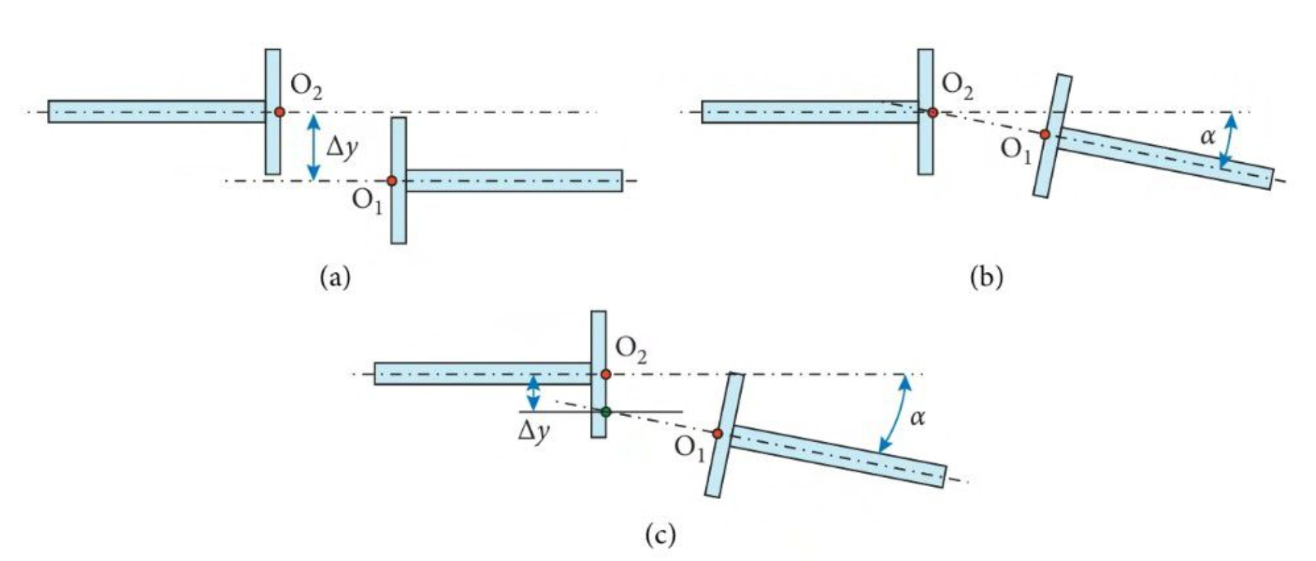
Figure 1: Types of misalignment. a) Parallel Misalignment b) Angular Misalignment c) Combined Misalignment.

Example 2.1: Rotor connected by a flexible mechanical coupling with parallel, angular or combined misalignment.

This example uses the rotor described in Section 1 to demonstrate the effects of a flexible coupling misalignment fault within the system.

"""Calculate the response of the rotor connected by a flexible mechanical coupling with parallel,
angular or combined misalignment."""
results_misalignment_flexible = rotor.run_misalignment(
    coupling="flex",
    mis_type="parallel",  # change here the type: mis_type="angular" or mis_type="combined"
    radial_stiffness=40e3,
    bending_stiffness=38e3,
    mis_distance_x=2e-4,
    mis_distance_y=2e-4,
    mis_angle=5 * np.pi / 180,
    input_torque=0,
    load_torque=0,
    n=0,
    speed=Q_(1200, "RPM"),
    node=node_unb,
    unbalance_magnitude=mass_unb,
    unbalance_phase=phase_unb,
    t=np.arange(0, 5, 0.0001),
    model_reduction={"num_modes": 12},  # Pseudo-modal method, optional
)

"""Plots the time response for the two given probes."""
results_misalignment_flexible.plot_1d([probe1, probe2]).show()